Ionic liquid with APPLE&P
APPLE&P is a polarizable force-field suitable for modeling electrolytes.
In this tutorial we will
create an initial structure of an ionic liquid,
perform atom typing suitable for the APPLE&P force field,
run a short APPLE&P barostat (NPT) simulation,
get the equilibrated density and a structure suitable as a starting point for further simulations
At the end, we will present some results and Python scripts for calculating the shear viscosity from long production simulations. Those properties can be extracted from APPLE&P simulations in the same way as for other AMS engines. See the Viscosity: Green-Kubo relation tutorial.
Good to know about APPLE&P: The bond lengths are constrained to values determined by the force field.
Create the initial ionic liquid system
Let’s start by creating the atomic structure with the Builder. We want to build a 1:1 mixture of
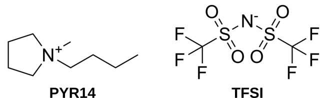
N-methyl-N-butylpyrrolidinium (pyr14)
bis(trifluoromethane sulfone imide) (TFSI)
If we do not specify a density, then one will automatically be estimated.
Experimental density at 333 K: 1.37 g/cm3
Estimated density by Builder: 1.04 g/cm3 (see below).
The estimated density is significantly lower than the experimental density. We will later equilibrate the density with a barostat simulation, so this is not a problem.
In fact, the lower density will make it easier
to generate the initial structure (pack the molecules), and
for the molecules to move around during the initial part of the MD simulation.
Note
The algorithm to estimate the density may change in future versions of AMS.
 →
→ 
0.9, or leave it empty and rely on the automatic estimation (will become 1.04).1350.CCCC[N+]1(CCCC1)C1.0 (default)cation to add another molecule
C(F)(F)(F)S(=O)(=O)[N-]S(=O)(=O)C(F)(F)F1.0 (default)anion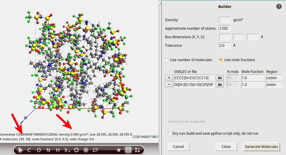
When using the Builder interface, the results are not always exact. To continue, we should double-check that the ratio of cation:anion really is 1:1, see the red arrow in the picture.
In this case, there are 30 PYR14 and 30 TFSI ions packed. Everything seems OK, so you may close the Builder window by clicking the Close button.
APPLE&P atom typing
Next we need to set up the APPLE&P engine and perform atom typing.
The APPLE&P atom typing tool
performs a connectivity analysis and identifies all atom types, and
writes a force field in your working directory with the extension .ff.
→  to go to the Model → APPLE&P panel.
+1 (pyr14)-1 (TFSI)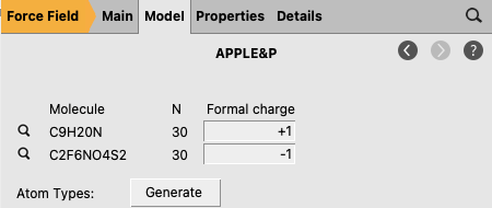
The message Finished generating APPLE&P atom types in the bottom-left corner of the molecule panel indicates that the atom typing was successful.
Note
If you enter incorrect charges, AMSinput will display an error message.
Molecular dynamics settings
The initial structure generated by the Builder is quite unrealistic:
the density is too low,
the packing does not take intermolecular interactions into account,
the bond lengths do not match the APPLE&P bond lengths
Typically, before running an NPT simulation with a barostat, it is a good idea to make the initial structure a bit more realistic, for example with a geometry optimization or short NVT simulation.
Here, we will instead just run a single simulation. The bond lengths will be automatically adjusted and kept fixed when the simulation starts.
MD Main panel
to go to the Model → MD panel.5000001.0 fs1000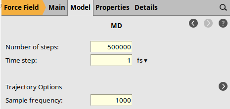
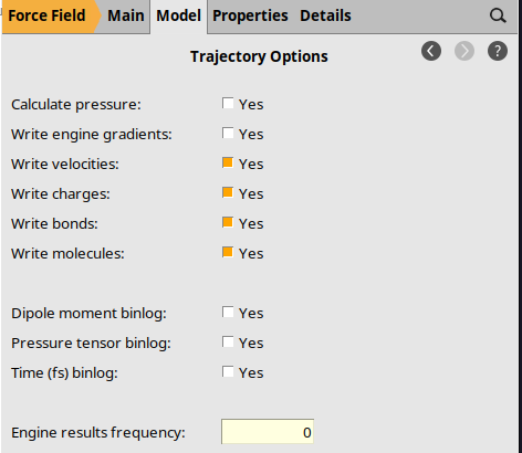
Trajectory Options
By default, AMS stores many engine results files on disk. For long MD simulations, these can take up a lot of disk space. For this simulation, we do not need them and can disable them:
0.
Thermostat Options
The initial structure is far from equilibrium, so we use the Berendsen thermostat and barostats.
to add a thermostat if none is visibleBerendsen333 K200 fs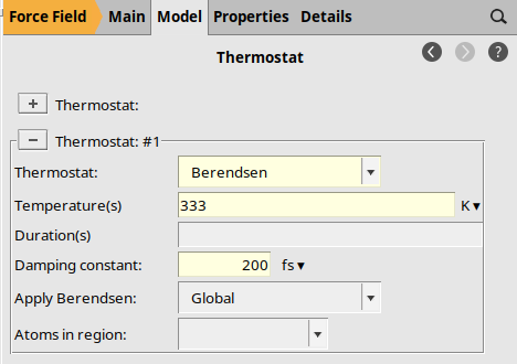
Barostat Options
The initial structure is far from equilibrium, so we use the Berendsen thermostat and barostats.
Berendsen1.0 bar5000 fs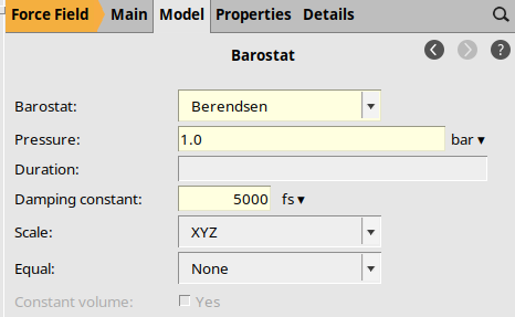
Run the MD simulation
This will run a 500 ps MD simulation. It may take several hours. You can visualize the progress in AMSmovie while the simulation is running.
Results: Equilibrated density
Your results should look something like this:
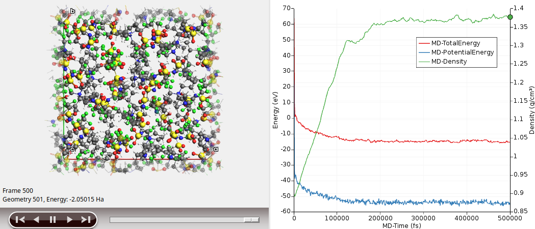
Here, we see that the density (green curve) seems to converge to a value of around 1.37 g/cm³ (experimental value: 1.37 g/cm³).
You may also more clearly visualize the cations and anions:
This highlights the cation and anion in red and green colors:
APPLE&P constrains the bond length
The distance will remain very nearly constant at 1.441 Å. All bond lengths are constrained to a distance determined by APPLE&P.
Compare to the input bond lengths:
 (or before AMS2026, if asked whether to update the geometry, select No)
What was the distance in the input system?
Note
The fact that APPLE&P constrains the bond lengths should be taken into account when modeling infinite (periodic) systems such as graphite/graphene. For such a system, the bond lengths in the initial geometry must match those in the force-field file before attempting to run energy minimization or molecular dynamics. Besides, unit cell dimensions that affect the constrained bonds must be frozen during optimization and MD. For example, for graphite/graphene this means that the xx, xy, and yy components of the strain have to be frozen.
Next steps
The structure from the final frame of the NPT simulation can be used for further simulations with more accurate simulation parameters. The structure is now close to equilibrium and therefore suitable to use with the NHC thermostat and MTK barostat.
Example: Computing viscosity
Below are some results for the calculated shear viscosity, from a long NVT simulation on the NPT-equilibrated density of this liquid:
Viscosity η (mPa s) [T = 333 K] |
|
Calculated with APPLE&P |
24 |
Experiment |
21 |
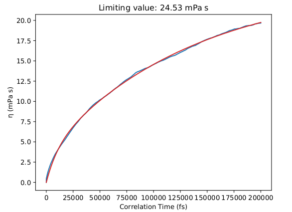
However, this simulation may take more than one week to complete so it is not part of this tutorial.
We obtain a good agreement with the experimental viscosity of the mixture equal to 21.0 mPa s (at 333 K, see Borodin 2009 and Tokuda et al.).
For details about how to calculate viscosity, see Viscosity: Green-Kubo relation.
Optional: Download a PLAMS Python workflow to run an entire workflow including
long NVT simulation, and then extract the viscosity with
viscosity_extractor.py
$AMSBIN/amspython applenp_viscosity_md.py
PYTHONUTF8=1 $AMSBIN/amspython viscosity_extractor.py /path/to/ams.rkf