Diffusion coefficient
In this tutorial we will compute the diffusion coefficients of Lithium ions in a Li0.4S cathode by means of molecular dynamics simulations with the ReaxFF engine.
The systems and workflows presented here are originally described in the publication ReaxFF molecular dynamics simulations on lithiated sulfur cathode materials Phys. Chem. Chem. Phys. 17, 3383-3393 (2015).
The tutorial consists of the following steps:
Importing a CIF file
Manipulating the structure (e.g. inserting particles) and equilibrating the system
Creating an amorphous structure by simulated annealing
Calculating diffusion coefficients from MD trajectories
If you wish, you can download the already-relaxed amorphous Li0.4S structure Li04S_amorphous.xyz and jump directly to the diffusion coefficient calculation
See also
Importing the Sulfur(α) crystal structure
 →
→ 
To speed up the calculations, we will use a smaller system than the one described in the publication. The crystal structure can be directly imported from a CIF file:
CIF file by clicking hereGenerating the Li0.4S system
We use the builder functionality of AMSinput to randomly insert 51 Li-atoms into our Sulfur system.
To insert single atoms, we use the SMILES code for a single Li atom: [Li] (including brackets).
See also
A better way of building the Li0.4S system is to use Grand Canonical Monte Carlo (GCMC). See also the Voltage profile from Grand-Canonical Monte Carlo tutorial.
[Li]51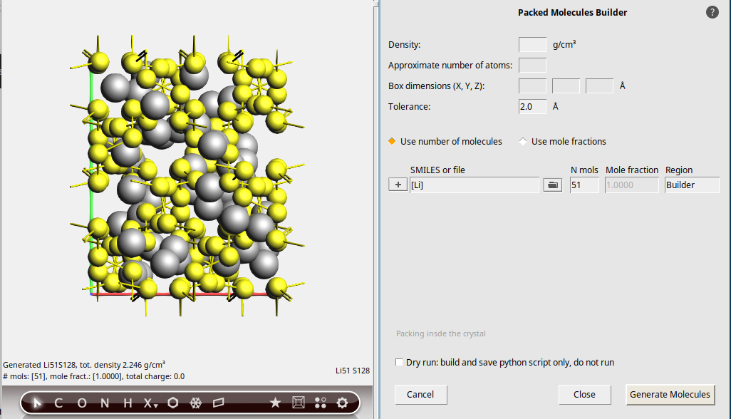
We now need to relax the geometry by running a geometry optimization including lattice relaxation:
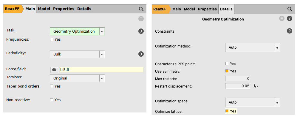
We are now ready to run the Li0.4S relaxation calculation:
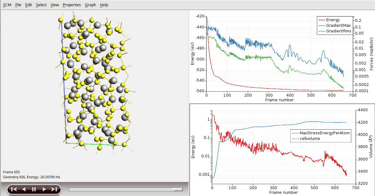
Note that the initial structure depends on random numbers, therefore your results may differ from the ones discussed here. The volume of the unit cell should have increased significantly during the optimization (here from about 3300 Å3 to about 4200 Å3):
Creating the amorphous systems by simulated annealing
Amorphous systems can be created with a Molecular Dynamics simulation by slowly heating up the system followed by a rapid cool-down.
As in the publication, we will anneal up to 1600 K followed by a rapid cool-down to room temperature. In order to speed up the calculation, only 30000 steps are calculated here.
 next to Task: Molecular Dynamics to go to the MD details
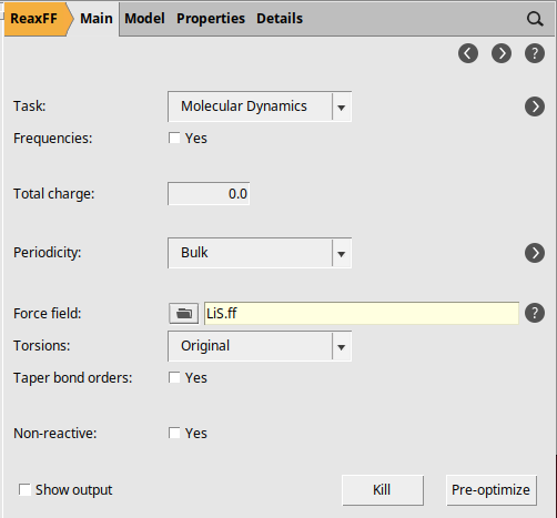
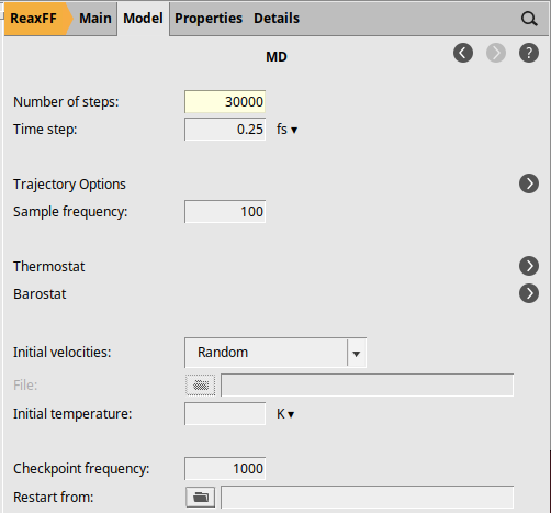
We will now set up the following temperature profile:
From start until step 5000: T = 300 K (constant)
From step 5000 to step 25000: heating up from 300 K to 1600 K
From step 25000 to step 30000: cooling down from 1600 K to 300 K
For more details on temperatures and pressure regimes, see the AMS manual on MD.
next to Thermostat to go to the thermostat details to add a new thermostat
300 300 1600 3005000 20000 5000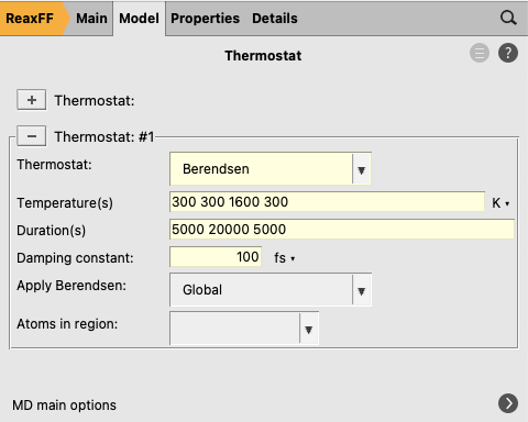
We are now ready to run the Li0.4S simulated annealing calculation:
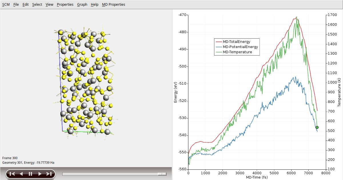
In AMSmovie you can follow the progress of the MD simulation, and you’ll be able to see the three temperature regimes:
We now need to relax the geometry of our new amorphous system by running a geometry optimization including lattice relaxation (as we did before):
Calculating the diffusion coefficients
We are now ready to run the final MD simulation to compute the Lithium diffusion coefficient D at T=1600 K.
You can calculate the diffusion coefficient in two different ways:
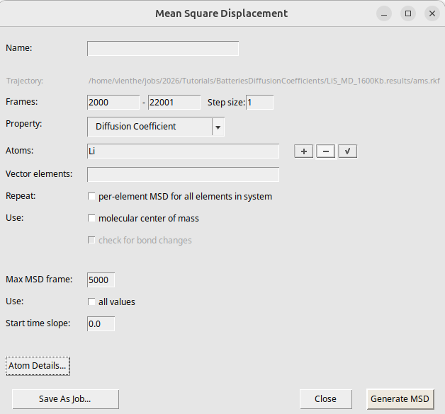
Through the slope of the mean squared displacement (MSD, recommended):
Through the integration of the velocity autocorrelation function (VACF, this requires setting sampling frequency to a small number):
Important
Because of finite-size effects, the diffusion coefficient depends on the size of the supercell (unless the supercell is very large). Typically, you would perform simulations for progressively larger supercells and extrapolate the calculated diffusion coefficients to the “infinite supercell” limit.
Set up and run the production simulation
Remark: if you did not create the amorphous structure yourself, but instead used the (already-relaxed) amorphous structure from the downloaded .xyz file, then first you may need to start AMSinput, select ReaxFF, and select the LiS.ff force field, and in one of the next steps you may need to add a new thermostat.
We will use a minimal proof-of-principle setup of 10000 equilibration steps followed by only 100000 production steps:
next to Task: Molecular Dynamics to go to the MD details next to Thermostat to go to the thermostat detailsTip
If you use the MSD to calculate the diffusion coefficient, you can set Sample frequency to a higher number (giving a smaller trajectory file).
Note
The time between two steps on the trajectory file will be sample_frequency * time_step = 5 * 0.25 fs = 1.25 fs.
We are now ready to run the calculation:
Diffusion coefficient through MSD (recommended)
After the calculation has finished, open it in AMSmovie:
Your results may look a bit different because of the short MD simulation and random initial velocities.
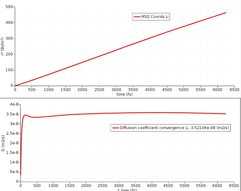
The MSD is the straight line in the above figure. If the MSD line is not straight, it means that you need to run a longer simulation to gather more statistics. It is calculated for times up to 6250 fs (controlled by the Max MSD Step option in the MSD window).
The other curve in the above figure shows the slope of the MSD divided by 6, calculated by performing a linear fit on the MSD from the “Start Time Slope” (that can be set in the MSD window) to each point on the MSD. The curve thus corresponds to the diffusion coefficient D. It should ideally be perfectly horizontal.
Note again that the initial structure and the MD simulation depends on random numbers, therefore your results may differ from the ones discussed here. Here, the curve seems to converge to a value around 3.52 × 10⁻⁸ m² s⁻¹.
Thus, D = 3.52 × 10⁻⁸ m² s⁻¹.
Diffusion coefficient through VACF
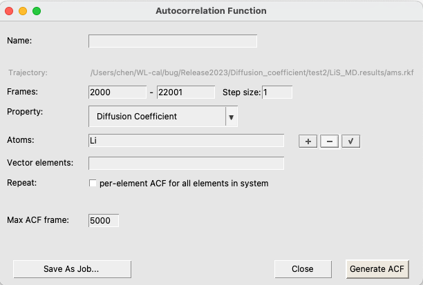
After the calculation is finished, we can obtain the Li diffusion coefficient by computing the velocity autocorrelation function for the Li atoms:
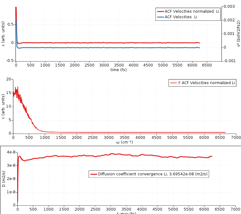
This plots
the velocity autocorrelation function,
the Fourier transform of the velocity autocorrelation function (power spectrum),
the integral of the velocity autocorrelation function divided by 3 (diffusion coefficient)
In this case, only the bottom plot is of interest to us. It should ideally become perfectly horizontal (converge) for large enough times.
Here, the value of the diffusion coefficient D = 3.70 × 10⁻⁸ m² s⁻¹ is approximately equal to the value obtained through the use of MSD analysis. Note that the initial structure and the MD simulation depends on random numbers, therefore your results may differ from the ones discussed here. However, the results with VACF should be close to the results with MSD, because they use the same MD trajectory.
Extrapolate to lower temperatures
Calculating the diffusion coefficient at 300K would require a very long trajectory. However, it is possible to provide an upper bound to the Li diffusion by means of extrapolation from elevated temperatures using the Arrhenius equation:
where \(D_0\) is the pre-exponential factor, \(E_a\) is the activation energy, \(k_B\) is the Boltzmann constant, and \(T\) is the temperature. The activation energy and pre-exponential factors can then be obtained from an Arrhenius plot of \(\ln{(D(T))}\) against \(1/T\). In order to extrapolate the diffusion coefficients for Li0.4S we calculate trajectories for at least four different temperatures (600 K, 800 K, 1200 K, 1600 K) for each system. One can then extrapolate the diffusion coefficient to lower temperature.
For an example on how to do this with a Python script, see Molecular Dynamics with Python.