NEB for Li diffusion in layered LiTiS2 (M3GNet)
Compute the minimum-energy Li migration pathway in periodic LiTiS2 with NEB using the M3GNet-UP-2022 potential and D3 dispersion. The workflow performs pristine relaxation, initial/final state preparation, NEB, barrier extraction, and profile plotting.
Li diffusion in layered LiTiS2 with NEB (M3GNet)
Self-contained notebook version of Part 2 of the NEB tutorial.
Workflow: 1. Relax pristine LiTiS2 (including lattice optimization). 2. Build and relax initial/final vacancy configurations. 3. Run NEB (19 images, 100 iterations) and extract diffusion barriers.
1) Define the pristine LiTiS2 structure
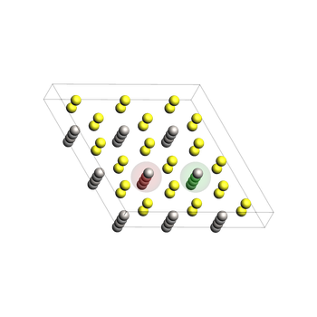
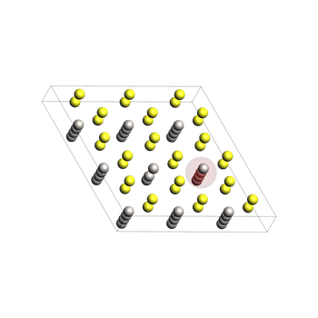
This is a supercell of the conventional crystal unit cell. It has been constructed from the optimized lattice.
To help with visualization, we add atoms 0 and 24 (zero-based indexing in Python), corresponding to atoms 1 and 25 in the GUI, to regions.
Later, we will remove Li atom 24 and visualize the diffusion of atom 0 into atom 24’s original position.
from scm.base import ChemicalSystem, Units
from scm.plams import view
litis2_pristine = ChemicalSystem(
"""
System
Lattice
10.314900000000 0.000000000000 0.000000000000
-5.157450000000 8.932965437496 0.000000000000
0.000000000000 0.000000000000 12.349810000000
End
Atoms
Li 1.719150000000 2.977655145832 6.174905000000
Ti 1.719150000000 2.977655145832 3.087452500000
S 1.719150000000 4.962758576353 4.551328274763
S 3.438300000000 3.970206861143 7.798481725237
Li 3.438300000000 5.955310291664 0.000000000000
Ti 3.438300000000 5.955310291664 9.262357500000
S 3.438300000000 7.940413722185 10.726233274763
S 5.157450000000 6.947862006975 1.623576725237
Li 3.438300000000 5.955310291664 6.174905000000
Ti 3.438300000000 5.955310291664 3.087452500000
S 3.438300000000 7.940413722185 4.551328274763
S 5.157450000000 6.947862006975 7.798481725237
Li 6.876600000000 0.000000000000 0.000000000000
Ti 6.876600000000 0.000000000000 9.262357500000
S 6.876600000000 1.985103430521 10.726233274763
S 8.595750000000 0.992551715311 1.623576725237
Li 6.876600000000 0.000000000000 6.174905000000
Ti 6.876600000000 0.000000000000 3.087452500000
S 6.876600000000 1.985103430521 4.551328274763
S 8.595750000000 0.992551715311 7.798481725237
Li 5.157450000000 2.977655145832 0.000000000000
Ti 5.157450000000 2.977655145832 9.262357500000
S 5.157450000000 4.962758576353 10.726233274763
S 6.876600000000 3.970206861143 1.623576725237
Li 5.157450000000 2.977655145832 6.174905000000
Ti 5.157450000000 2.977655145832 3.087452500000
S 5.157450000000 4.962758576353 4.551328274763
S 6.876600000000 3.970206861143 7.798481725237
Li -3.438300000000 5.955310291664 0.000000000000
Ti -3.438300000000 5.955310291664 9.262357500000
S -3.438300000000 7.940413722185 10.726233274763
S -1.719150000000 6.947862006975 1.623576725237
Li -3.438300000000 5.955310291664 6.174905000000
Ti -3.438300000000 5.955310291664 3.087452500000
S -3.438300000000 7.940413722185 4.551328274763
S -1.719150000000 6.947862006975 7.798481725237
Li 0.000000000000 0.000000000000 0.000000000000
Ti 0.000000000000 0.000000000000 9.262357500000
S 0.000000000000 1.985103430521 10.726233274763
S 1.719150000000 0.992551715311 1.623576725237
Li 0.000000000000 0.000000000000 6.174905000000
Ti 0.000000000000 0.000000000000 3.087452500000
S 0.000000000000 1.985103430521 4.551328274763
S 1.719150000000 0.992551715311 7.798481725237
Li -1.719150000000 2.977655145832 0.000000000000
Ti -1.719150000000 2.977655145832 9.262357500000
S -1.719150000000 4.962758576353 10.726233274763
S 0.000000000000 3.970206861143 1.623576725237
Li -1.719150000000 2.977655145832 6.174905000000
Ti -1.719150000000 2.977655145832 3.087452500000
S -1.719150000000 4.962758576353 4.551328274763
S 0.000000000000 3.970206861143 7.798481725237
Li 0.000000000000 5.955310291664 0.000000000000
Ti 0.000000000000 5.955310291664 9.262357500000
S 0.000000000000 7.940413722185 10.726233274763
S 1.719150000000 6.947862006975 1.623576725237
Li 0.000000000000 5.955310291664 6.174905000000
Ti 0.000000000000 5.955310291664 3.087452500000
S 0.000000000000 7.940413722185 4.551328274763
S 1.719150000000 6.947862006975 7.798481725237
Li 3.438300000000 0.000000000000 0.000000000000
Ti 3.438300000000 0.000000000000 9.262357500000
S 3.438300000000 1.985103430521 10.726233274763
S 5.157450000000 0.992551715311 1.623576725237
Li 3.438300000000 0.000000000000 6.174905000000
Ti 3.438300000000 0.000000000000 3.087452500000
S 3.438300000000 1.985103430521 4.551328274763
S 5.157450000000 0.992551715311 7.798481725237
Li 1.719150000000 2.977655145832 0.000000000000
Ti 1.719150000000 2.977655145832 9.262357500000
S 1.719150000000 4.962758576353 10.726233274763
S 3.438300000000 3.970206861143 1.623576725237
End
End
"""
)
# zero-based indexing
diffusing_atom = 0
to_be_removed_atom = 24
litis2_pristine.set_atoms_in_region([diffusing_atom], "diffusing_atom")
litis2_pristine.set_atoms_in_region([to_be_removed_atom], "to_be_removed_atom")
view(litis2_pristine, width=350, height=350, direction="tilt_c", show_regions=True)
[10.04|12:20:45] Starting Xvfb...
[10.04|12:20:45] Xvfb started
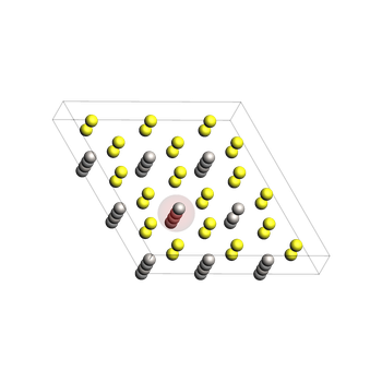
4) Build and relax the initial vacancy state
Remove the Li atom (GUI index 25 -> Python index 24) to create a vacancy.
Initial system (before relaxation)
sys_init = litis2_pristine.copy()
# important: we will remove atoms so we need to create an unrelated copy (here a list) of the coordinates to save
# otherwise the value of coords_target will change when we remove the atom
coords_target = list(sys_init.atoms[to_be_removed_atom].coords)
sys_init.remove_atom(to_be_removed_atom)
print(f"The atom will diffuse from {sys_init.atoms[diffusing_atom].coords} to {coords_target}")
view(sys_init, width=350, height=350, direction="tilt_c", show_regions=True)
The atom will diffuse from [1.71915 2.97765515 6.174905 ] to [5.15745, 2.977655145832, 6.174905]
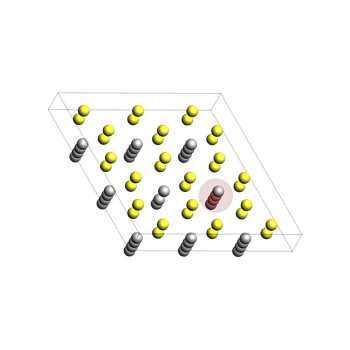
The final system (before relaxation)
Move the hopping Li atom to the vacancy site (GUI index 1 -> Python index 0)
sys_final = sys_init.copy()
sys_final.atoms[diffusing_atom].coords = coords_target
view(sys_final, width=350, height=350, direction="tilt_c", show_regions=True)
sett_opt = plams.Settings()
sett_opt.input.ams.Task = "GeometryOptimization"
sett_opt.input.ams.GeometryOptimization.OptimizeLattice = "No"
job_init = plams.AMSJob(
settings=sett_opt + make_engine_settings(),
molecule=sys_init,
name="LiTiS2_init",
)
job_init.run()
job_final = plams.AMSJob(
settings=sett_opt + make_engine_settings(),
molecule=sys_final,
name="LiTiS2_final",
)
job_final.run()
plams.log(f"{job_init.ok()=}, {job_final.ok()=}")
assert job_final.ok(), "Final-state optimization FAILED"
[10.04|12:20:48] JOB LiTiS2_init STARTED
[10.04|12:20:48] JOB LiTiS2_init RUNNING
[10.04|12:20:57] JOB LiTiS2_init FINISHED
[10.04|12:20:57] JOB LiTiS2_init SUCCESSFUL
[10.04|12:20:57] JOB LiTiS2_final STARTED
[10.04|12:20:57] JOB LiTiS2_final RUNNING
[10.04|12:21:05] JOB LiTiS2_final FINISHED
[10.04|12:21:05] JOB LiTiS2_final SUCCESSFUL
[10.04|12:21:05] job_init.ok()=True, job_final.ok()=True
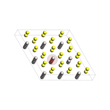
Relaxed initial geometry:job_final
relaxed_init = job_init.results.get_main_system()
view(relaxed_init, width=350, height=350, direction="tilt_c", show_regions=True)
Relaxed final geometry:
relaxed_final = job_final.results.get_main_system()
view(relaxed_final, width=350, height=350, direction="tilt_c", show_regions=True)
6) Run the NEB calculation
Use optimized initial/final systems with 19 images and 100 iterations.
sett_neb = plams.Settings()
sett_neb.input.ams.Task = "NEB"
sett_neb.input.ams.NEB.Images = 19
sett_neb.input.ams.NEB.Iterations = 100
neb_systems = {"": relaxed_init, "final": relaxed_final}
job_neb = plams.AMSJob(
settings=sett_neb + make_engine_settings(),
molecule=neb_systems,
name="LiTiS2_NEB",
)
res_neb = job_neb.run()
assert job_neb.ok(), "NEB calculation FAILED"
print(f"{job_neb.name}: OK")
[10.04|12:21:07] JOB LiTiS2_NEB STARTED
[10.04|12:21:07] JOB LiTiS2_NEB RUNNING
[10.04|12:22:33] JOB LiTiS2_NEB FINISHED
[10.04|12:22:33] JOB LiTiS2_NEB SUCCESSFUL
LiTiS2_NEB: OK
7) Extract NEB results and barriers
Print NEB summary data and convert left/right barriers from Hartree to eV.
from pprint import pprint
assert job_neb.ok(), "Looks like NEB calculation failed?"
neb_res = res_neb.get_neb_results()
pprint(neb_res)
ha2ev = Units.conversion_factor("hartree", "eV")
left_barrier_ev = neb_res["LeftBarrier"] * ha2ev
right_barrier_ev = neb_res["RightBarrier"] * ha2ev
print(f"Left TS barrier : {left_barrier_ev:.6f} eV")
print(f"Right TS barrier: {right_barrier_ev:.6f} eV")
{'Climbing': True,
'Energies': [-16.564932431837118,
-16.564867480657007,
-16.56402543475297,
-16.562632969358706,
-16.56075920164935,
-16.55855629234889,
-16.556233613906592,
-16.554024662385785,
-16.552165529324235,
-16.55093315338219,
-16.55050575343035,
-16.550933153320546,
-16.552165530379597,
-16.554024663519893,
... output trimmed ....
Molecule('Li17S36Ti18' at 0x16b81ad60),
Molecule('Li17S36Ti18' at 0x16b819bb0),
Molecule('Li17S36Ti18' at 0x16b821a00),
Molecule('Li17S36Ti18' at 0x16b870850),
Molecule('Li17S36Ti18' at 0x16b84e700),
Molecule('Li17S36Ti18' at 0x16b883550),
Molecule('Li17S36Ti18' at 0x16b8873a0),
Molecule('Li17S36Ti18' at 0x16b8921f0),
Molecule('Li17S36Ti18' at 0x16b8b1070)],
'ReactionEnergy': -2.2964741219766438e-10,
'RightBarrier': 0.014426678636414891,
'nImages': 19,
'nIterations': 100}
Left TS barrier : 0.392570 eV
Right TS barrier: 0.392570 eV
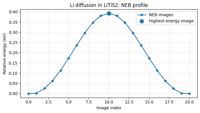
8) Plot the NEB energy profile
Plot relative image energies (eV) and mark the highest-energy image.
import matplotlib.pyplot as plt
neb_res = res_neb.get_neb_results()
energies_au = neb_res["Energies"]
ha2ev = Units.conversion_factor("hartree", "eV")
energies_ev = [e * ha2ev for e in energies_au]
ref = energies_ev[0]
rel_ev = [e - ref for e in energies_ev]
x = list(range(len(rel_ev)))
hi = neb_res["HighestIndex"]
fig, ax = plt.subplots(figsize=(7, 4))
ax.plot(x, rel_ev, "-o", lw=1.8, ms=5, label="NEB images")
ax.scatter([hi], [rel_ev[hi]], s=90, zorder=3, label="Highest-energy image")
ax.set_xlabel("Image index")
ax.set_ylabel("Relative energy (eV)")
ax.set_title("Li diffusion in LiTiS2: NEB profile")
ax.grid(alpha=0.3)
ax.legend()
fig.tight_layout()
ax
print(f"Left barrier (eV): {neb_res['LeftBarrier'] * ha2ev:.6f}")
print(f"Right barrier (eV): {neb_res['RightBarrier'] * ha2ev:.6f}")
print(f"Highest image index: {hi}")
Left barrier (eV): 0.392570
Right barrier (eV): 0.392570
Highest image index: 10
See also
Python Script
#!/usr/bin/env python
# coding: utf-8
# ## Li diffusion in layered LiTiS2 with NEB (M3GNet)
#
# Self-contained notebook version of Part 2 of the NEB tutorial.
#
# Workflow:
# 1. Relax pristine LiTiS2 (including lattice optimization).
# 2. Build and relax initial/final vacancy configurations.
# 3. Run NEB (`19` images, `100` iterations) and extract diffusion barriers.
#
# ### 2) Initialize PLAMS and define shared engine helper
#
# Set up the PLAMS work folder and a helper that returns M3GNet+D3 settings with single-process/thread execution.
#
import scm.plams as plams

plams.init(folder="LiTiS2_NEB")


def make_engine_settings():
    s = plams.Settings()
    s.runscript.nproc = 1
    s.runscript.preamble_lines = ["export OMP_NUM_THREADS=1"]
    s.input.MLPotential.Backend = "M3GNet"
    s.input.MLPotential.Model = "M3GNet-UP-2022"
    s.input.ams.EngineAddons.D3Dispersion.Enabled = "Yes"
    return s
# ### 1) Define the pristine LiTiS2 structure
#
# This is a supercell of the conventional crystal unit cell. It has been constructed from the optimized lattice.
#
# To help with visualization, we add atoms 0 and 24 (zero-based indexing in Python), corresponding to atoms 1 and 25 in the GUI, to regions.
#
# Later, we will remove Li atom 24 and visualize the diffusion of atom 0 into atom 24's original position.
#
from scm.base import ChemicalSystem, Units
from scm.plams import view
litis2_pristine = ChemicalSystem(
"""
System
Lattice
10.314900000000 0.000000000000 0.000000000000
-5.157450000000 8.932965437496 0.000000000000
0.000000000000 0.000000000000 12.349810000000
End
Atoms
Li 1.719150000000 2.977655145832 6.174905000000
Ti 1.719150000000 2.977655145832 3.087452500000
S 1.719150000000 4.962758576353 4.551328274763
S 3.438300000000 3.970206861143 7.798481725237
Li 3.438300000000 5.955310291664 0.000000000000
Ti 3.438300000000 5.955310291664 9.262357500000
S 3.438300000000 7.940413722185 10.726233274763
S 5.157450000000 6.947862006975 1.623576725237
Li 3.438300000000 5.955310291664 6.174905000000
Ti 3.438300000000 5.955310291664 3.087452500000
S 3.438300000000 7.940413722185 4.551328274763
S 5.157450000000 6.947862006975 7.798481725237
Li 6.876600000000 0.000000000000 0.000000000000
Ti 6.876600000000 0.000000000000 9.262357500000
S 6.876600000000 1.985103430521 10.726233274763
S 8.595750000000 0.992551715311 1.623576725237
Li 6.876600000000 0.000000000000 6.174905000000
Ti 6.876600000000 0.000000000000 3.087452500000
S 6.876600000000 1.985103430521 4.551328274763
S 8.595750000000 0.992551715311 7.798481725237
Li 5.157450000000 2.977655145832 0.000000000000
Ti 5.157450000000 2.977655145832 9.262357500000
S 5.157450000000 4.962758576353 10.726233274763
S 6.876600000000 3.970206861143 1.623576725237
Li 5.157450000000 2.977655145832 6.174905000000
Ti 5.157450000000 2.977655145832 3.087452500000
S 5.157450000000 4.962758576353 4.551328274763
S 6.876600000000 3.970206861143 7.798481725237
Li -3.438300000000 5.955310291664 0.000000000000
Ti -3.438300000000 5.955310291664 9.262357500000
S -3.438300000000 7.940413722185 10.726233274763
S -1.719150000000 6.947862006975 1.623576725237
Li -3.438300000000 5.955310291664 6.174905000000
Ti -3.438300000000 5.955310291664 3.087452500000
S -3.438300000000 7.940413722185 4.551328274763
S -1.719150000000 6.947862006975 7.798481725237
Li 0.000000000000 0.000000000000 0.000000000000
Ti 0.000000000000 0.000000000000 9.262357500000
S 0.000000000000 1.985103430521 10.726233274763
S 1.719150000000 0.992551715311 1.623576725237
Li 0.000000000000 0.000000000000 6.174905000000
Ti 0.000000000000 0.000000000000 3.087452500000
S 0.000000000000 1.985103430521 4.551328274763
S 1.719150000000 0.992551715311 7.798481725237
Li -1.719150000000 2.977655145832 0.000000000000
Ti -1.719150000000 2.977655145832 9.262357500000
S -1.719150000000 4.962758576353 10.726233274763
S 0.000000000000 3.970206861143 1.623576725237
Li -1.719150000000 2.977655145832 6.174905000000
Ti -1.719150000000 2.977655145832 3.087452500000
S -1.719150000000 4.962758576353 4.551328274763
S 0.000000000000 3.970206861143 7.798481725237
Li 0.000000000000 5.955310291664 0.000000000000
Ti 0.000000000000 5.955310291664 9.262357500000
S 0.000000000000 7.940413722185 10.726233274763
S 1.719150000000 6.947862006975 1.623576725237
Li 0.000000000000 5.955310291664 6.174905000000
Ti 0.000000000000 5.955310291664 3.087452500000
S 0.000000000000 7.940413722185 4.551328274763
S 1.719150000000 6.947862006975 7.798481725237
Li 3.438300000000 0.000000000000 0.000000000000
Ti 3.438300000000 0.000000000000 9.262357500000
S 3.438300000000 1.985103430521 10.726233274763
S 5.157450000000 0.992551715311 1.623576725237
Li 3.438300000000 0.000000000000 6.174905000000
Ti 3.438300000000 0.000000000000 3.087452500000
S 3.438300000000 1.985103430521 4.551328274763
S 5.157450000000 0.992551715311 7.798481725237
Li 1.719150000000 2.977655145832 0.000000000000
Ti 1.719150000000 2.977655145832 9.262357500000
S 1.719150000000 4.962758576353 10.726233274763
S 3.438300000000 3.970206861143 1.623576725237
End
End
"""
)
# zero-based indexing
diffusing_atom = 0
to_be_removed_atom = 24
litis2_pristine.set_atoms_in_region([diffusing_atom], "diffusing_atom")
litis2_pristine.set_atoms_in_region([to_be_removed_atom], "to_be_removed_atom")
view(litis2_pristine, width=350, height=350, direction="tilt_c", show_regions=True, picture_path="picture1.png")
# ### 4) Build and relax the initial vacancy state
#
# Remove the Li atom (GUI index 25 -> Python index 24) to create a vacancy.
#
# #### Initial system (before relaxation)
sys_init = litis2_pristine.copy()
# important: we will remove atoms so we need to create an unrelated copy (here a list) of the coordinates to save
# otherwise the value of coords_target will change when we remove the atom
coords_target = list(sys_init.atoms[to_be_removed_atom].coords)
sys_init.remove_atom(to_be_removed_atom)
print(f"The atom will diffuse from {sys_init.atoms[diffusing_atom].coords} to {coords_target}")
view(sys_init, width=350, height=350, direction="tilt_c", show_regions=True, picture_path="picture2.png")
# #### The final system (before relaxation)
#
# Move the hopping Li atom to the vacancy site (GUI index 1 -> Python index 0)
sys_final = sys_init.copy()
sys_final.atoms[diffusing_atom].coords = coords_target
view(sys_final, width=350, height=350, direction="tilt_c", show_regions=True, picture_path="picture3.png")
sett_opt = plams.Settings()
sett_opt.input.ams.Task = "GeometryOptimization"
sett_opt.input.ams.GeometryOptimization.OptimizeLattice = "No"


job_init = plams.AMSJob(
    settings=sett_opt + make_engine_settings(),
    molecule=sys_init,
    name="LiTiS2_init",
)
job_init.run()

job_final = plams.AMSJob(
    settings=sett_opt + make_engine_settings(),
    molecule=sys_final,
    name="LiTiS2_final",
)
job_final.run()

plams.log(f"{job_init.ok()=}, {job_final.ok()=}")
assert job_final.ok(), "Final-state optimization FAILED"
# #### Relaxed initial geometry:job_final
relaxed_init = job_init.results.get_main_system()
view(relaxed_init, width=350, height=350, direction="tilt_c", show_regions=True, picture_path="picture4.png")
# #### Relaxed final geometry:
relaxed_final = job_final.results.get_main_system()
view(relaxed_final, width=350, height=350, direction="tilt_c", show_regions=True, picture_path="picture5.png")
# ### 6) Run the NEB calculation
#
# Use optimized initial/final systems with 19 images and 100 iterations.
#
sett_neb = plams.Settings()
sett_neb.input.ams.Task = "NEB"
sett_neb.input.ams.NEB.Images = 19
sett_neb.input.ams.NEB.Iterations = 100

neb_systems = {"": relaxed_init, "final": relaxed_final}

job_neb = plams.AMSJob(
    settings=sett_neb + make_engine_settings(),
    molecule=neb_systems,
    name="LiTiS2_NEB",
)
res_neb = job_neb.run()

assert job_neb.ok(), "NEB calculation FAILED"
print(f"{job_neb.name}: OK")
# ### 7) Extract NEB results and barriers
#
# Print NEB summary data and convert left/right barriers from Hartree to eV.
#
from pprint import pprint

assert job_neb.ok(), "Looks like NEB calculation failed?"

neb_res = res_neb.get_neb_results()
pprint(neb_res)

ha2ev = Units.conversion_factor("hartree", "eV")
left_barrier_ev = neb_res["LeftBarrier"] * ha2ev
right_barrier_ev = neb_res["RightBarrier"] * ha2ev

print(f"Left TS barrier : {left_barrier_ev:.6f} eV")
print(f"Right TS barrier: {right_barrier_ev:.6f} eV")
# ### 8) Plot the NEB energy profile
#
# Plot relative image energies (eV) and mark the highest-energy image.
#
import matplotlib.pyplot as plt

neb_res = res_neb.get_neb_results()
energies_au = neb_res["Energies"]
ha2ev = Units.conversion_factor("hartree", "eV")
energies_ev = [e * ha2ev for e in energies_au]

ref = energies_ev[0]
rel_ev = [e - ref for e in energies_ev]

x = list(range(len(rel_ev)))
hi = neb_res["HighestIndex"]

fig, ax = plt.subplots(figsize=(7, 4))
ax.plot(x, rel_ev, "-o", lw=1.8, ms=5, label="NEB images")
ax.scatter([hi], [rel_ev[hi]], s=90, zorder=3, label="Highest-energy image")
ax.set_xlabel("Image index")
ax.set_ylabel("Relative energy (eV)")
ax.set_title("Li diffusion in LiTiS2: NEB profile")
ax.grid(alpha=0.3)
ax.legend()
fig.tight_layout()
ax
print(f"Left barrier  (eV): {neb_res['LeftBarrier'] * ha2ev:.6f}")
print(f"Right barrier (eV): {neb_res['RightBarrier'] * ha2ev:.6f}")
print(f"Highest image index: {hi}")