Active Learning: Li-Vacancy Diffusion NEB in LiTiS2
Train an M3GNet model for Li-vacancy migration in LiTiS2.
Initialization
import scm.plams as plams
import os
import numpy as np
import matplotlib.pyplot as plt
import scm.params as params
from scm.simple_active_learning import SimpleActiveLearningJob
plams.init()
PLAMS working folder: /path/to/plams_workdir.007
Create structures
Create primitive cell from coordinates
# for plotting in Jupyter notebooks
rotation = "-85x,-5y,0z"

# create structure
primitive = plams.AMSJob.from_input(
    """
    System
        Atoms
            Li 0. 0. 0.
            Ti 0. 0. 3.087452499999999
            S 0. 1.985103430533333 4.551328274799999
            S 1.71915 0.9925517153000001 1.6235767252
        End
        Lattice
            3.4383 0.0 0.0
            -1.71915 2.977655145833333 0.0
            0.0 0.0 6.174905
        End
    End
"""
).molecule[""]
plams.plot_molecule(primitive, rotation=rotation)

Create a supercell.
Here we a reasonably-sized supercell. If the cell is very small, it is actually quite inefficient for training the machine learning potential. If every atom sees its own periodic image then there will not be sufficient variety in the atomic environments for the ML potential to be able to extrapolate to unseen environments. It is recommended to use a larger supercell.
supercell = primitive.supercell([[3, 0, 0], [2, 4, 0], [0, 0, 2]])
for at in supercell:
    at.properties = plams.Settings()
plams.plot_molecule(supercell, rotation=rotation)
print("Lattice vectors")
print(supercell.lattice)
print(f"Number of atoms: {len(supercell)}")
Lattice vectors
[(10.3149, 0.0, 0.0), (0.0, 11.910620583333332, 0.0), (0.0, 0.0, 12.34981)]
Number of atoms: 96
Create Li vacancy in two different places
li_indices = [i for i, at in enumerate(supercell, 1) if at.symbol == "Li"]
print(f"Li indices (starting with 1): {li_indices}")
Li indices (starting with 1): [1, 5, 9, 13, 17, 21, 25, 29, 33, 37, 41, 45, 49, 53, 57, 61, 65, 69, 73, 77, 81, 85, 89, 93]
Pick the first Li atom, and get its nearest Li neighbor.
Note that the PLAMS distance_to function ignores periodic boundary conditions, which in this case is quite convenient as it will make the visualization easier if the Li atom diffuses inside the unit cell and doesn’t cross the periodic boundary.
first_index = li_indices[0]
li1 = supercell[first_index]
li1.properties.region = "DiffusingLi"
distances = [li1.distance_to(supercell[x]) for x in li_indices[1:]]
nearest_neighbor_index = li_indices[np.argmin(distances) + 1]
li2 = supercell[nearest_neighbor_index]
target_coords = li2.coords
print(f"First Li atom: {li1}")
print(f"Second Li atom: {li2}")
First Li atom:         Li       0.000000       0.000000       0.000000
Second Li atom:         Li       3.438300       0.000000       0.000000
The goal is to make a Li atom diffuse between these two positions.
For this, we will first delete the second Li atom, and then create a new structure in which the first Li atom is translated to the second Li atom coordinates.
defective_1 = supercell.copy()
defective_1.delete_atom(defective_1[nearest_neighbor_index])
defective_2 = supercell.copy()
defective_2.delete_atom(defective_2[nearest_neighbor_index])
defective_2[first_index].coords = li2.coords
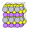
plams.plot_molecule(defective_1, rotation=rotation)
plt.title("Initial structure");

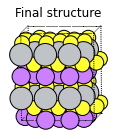
The Li atom in the bottom left corner will diffuse to the right (the vacancy will diffuse to the left):
plams.plot_molecule(defective_2, rotation=rotation)
plt.title("Final structure");
Initial validation of diffusion barrier with NEB and M3GNet-UP-2022
M3GNet-UP-2022 NEB job
m3gnet_up_s = plams.Settings()
m3gnet_up_s.input.MLPotential.Model = "M3GNet-UP-2022"

neb_s = plams.Settings()
neb_s.input.ams.Task = "NEB"
neb_s.input.ams.NEB.PreoptimizeWithIDPP = "Yes"
neb_s.input.ams.NEB.Images = 7
m3gnet_up_neb_job = plams.AMSJob(
    settings=m3gnet_up_s + neb_s,
    molecule={"": defective_1, "final": defective_2},
    name="m3gnet_up_neb",
)
m3gnet_up_neb_job.run();
[25.03|10:51:33] JOB m3gnet_up_neb STARTED
[25.03|10:51:33] JOB m3gnet_up_neb RUNNING
[25.03|10:51:58] JOB m3gnet_up_neb FINISHED
[25.03|10:51:58] JOB m3gnet_up_neb SUCCESSFUL
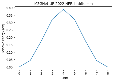
M3GNet-UP-2022 NEB results
m3gnet_up_res = m3gnet_up_neb_job.results.get_neb_results(unit="eV")
print(f"Left barrier: {m3gnet_up_res['LeftBarrier']:.3f} eV")
print(f"Right barrier: {m3gnet_up_res['RightBarrier']:.3f} eV")
Left barrier: 0.388 eV
Right barrier: 0.388 eV
# ref_results = [0.0, 0.144, 0.482, 0.816, 0.963, 0.816, 0.482, 0.144, 0.0]  # from Quantum ESPRESSO DFT calculation
nImages = m3gnet_up_res["nImages"]
relative_energies = np.array(m3gnet_up_res["Energies"]) - m3gnet_up_res["Energies"][0]
plt.plot(relative_energies)
plt.xlabel("Image")
plt.ylabel("Relative energy (eV)")
plt.title("M3GNet-UP-2022 NEB Li diffusion");
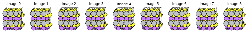
fig, axes = plt.subplots(1, len(m3gnet_up_res["Molecules"]), figsize=(15, 5))

for i, mol in enumerate(m3gnet_up_res["Molecules"]):
    plams.plot_molecule(mol, ax=axes[i], rotation=rotation)
    axes[i].set_title(f"Image {i}")
!amsmovie "{m3gnet_up_neb_job.results.rkfpath()}"
DFT reference engine settings
Are the above M3GNet-UP-2022 results any good? Let’s compare to DFT calculations using the AMS “Replay” task.
“Replay” is just a series of singlepoints on the previous NEB structures. It is not a NEB calculation.
Here we use the Quantum ESPRESSO engine available in AMS2024.
dft_s = plams.Settings()
dft_s.input.QuantumESPRESSO.System.occupations = "Smearing"
dft_s.input.QuantumESPRESSO.System.degauss = 0.005
# for production purposes always manually check that ecutwfc and ecutrho are high enough
# here we set a fairly low ecutwfc to speed up the calculation
dft_s.input.QuantumESPRESSO.System.ecutwfc = 30.0
dft_s.input.QuantumESPRESSO.System.ecutrho = 240.0
# decrease mixing_beta for more robust SCF convergence
dft_s.input.QuantumESPRESSO.Electrons.mixing_beta = 0.3
dft_s.input.QuantumESPRESSO.Electrons.conv_thr = 1.0e-5 * len(supercell)
# for a small cell one should ideally use more k-points than just the gamma point
# by settings K_Points._h = "gamma" we use the faster gamma-point-only
# implementation in Quantum ESPRESSO
dft_s.input.QuantumESPRESSO.K_Points._h = "gamma"
# SCM_DISABLE_MPI launches ams in serial, but will still run Quantum ESPRESSO in parallel
dft_s.runscript.preamble_lines = ["export SCM_DISABLE_MPI=1"]
Run DFT calculations on the NEB points from M3GNet-UP-2022
Note: The DFT calculations may take a few minutes to complete.
replay_s = plams.Settings()
replay_s.input.ams.Task = "Replay"
replay_s.input.ams.Replay.File = os.path.abspath(m3gnet_up_neb_job.results.rkfpath())
replay_s.input.ams.Properties.Gradients = "Yes"

replay_dft_job = plams.AMSJob(
    settings=replay_s + dft_s, name="replay_m3gnet_up_neb_with_dft"
)
replay_dft_job.run(watch=True);
[25.03|10:52:07] JOB replay_m3gnet_up_neb_with_dft STARTED
[25.03|10:52:07] JOB replay_m3gnet_up_neb_with_dft RUNNING
[25.03|10:52:07] replay_m3gnet_up_neb_with_dft: AMS 2024.101  RunTime: Mar25-2024 10:52:07  ShM Nodes: 1  Procs: 1
[25.03|10:52:07] replay_m3gnet_up_neb_with_dft: Starting trajectory replay ...
[25.03|10:52:07] replay_m3gnet_up_neb_with_dft: Replaying frame #1/9 (#342 in original trajectory)
... output trimmed ....
[25.03|11:05:27] replay_m3gnet_up_neb_with_dft: Trajectory replay complete.
[25.03|11:05:27] replay_m3gnet_up_neb_with_dft: Number of QE evaluations: 9
[25.03|11:05:27] replay_m3gnet_up_neb_with_dft: NORMAL TERMINATION
[25.03|11:05:27] JOB replay_m3gnet_up_neb_with_dft FINISHED
[25.03|11:05:27] JOB replay_m3gnet_up_neb_with_dft SUCCESSFUL
When using “Replay” on a NEB job, the results are stored in the normal NEB format. Thus we can use the .get_neb_results() method also on this job:
dft_energies = replay_dft_job.results.get_neb_results(unit="eV")["Energies"]
dft_relative_energies = np.array(dft_energies) - dft_energies[0]

plt.plot(relative_energies)
plt.plot(dft_relative_energies)
plt.legend(["M3GNet-UP-2022", "DFT singlepoints"])
plt.title("Compare M3GNet-UP-2022 NEB to DFT singlepoints");
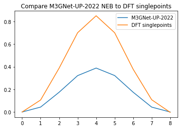
Conclusion: M3GNet-UP-2022 significantly underestimates the diffusion barrier compared to DFT calculations. This motivates the reparametrization
Store DFT results for later
Since we already performed some DFT calculations, we may as well add them to the training set.
ri = params.ResultsImporter(
    settings={"units": {"energy": "eV", "forces": "eV/angstrom"}}
)
ri.add_trajectory_singlepoints(
    replay_dft_job,
    properties=["energy", "forces"],
    indices=[0, 1, 2, 3, 4],
    data_set="training_set",
)
ri.add_trajectory_singlepoints(
    replay_dft_job,
    properties=["energy", "forces"],
    indices=[5],
    data_set="validation_set",
)
yaml_dir = "lidiffusion_initial_reference_data"
ri.store(yaml_dir, backup=False)
['lidiffusion_initial_reference_data/job_collection.yaml',
 'lidiffusion_initial_reference_data/results_importer_settings.yaml',
 'lidiffusion_initial_reference_data/training_set.yaml',
 'lidiffusion_initial_reference_data/validation_set.yaml']
Preliminary active learning jobs with equilibrium MD
Let’s first run some simple NVT MD with active learning for both the * stochiometric system (supercell), and * defective system (defective_1)
This is just to get a good general sampling before setting up the reaction boost to explicitly sample the diffusion process.
Active Learning for stoichiometric system
The stoichiometric system is a perfect crystal with not so many atoms. The forces will be very close to 0 also after a few MD frames. However, even if the ML model predicts forces close to 0, the R^2 between predicted and reference forces may be quite low.
In a case like this, it is reasonable to either
decrease the MinR2 success criterion, and/or
perturb the atomic coordinates of the initial structure a bit, so that the forces aren’t extremely small
Here, we do both of these:
nvt_md_s = plams.AMSNVTJob(
    nsteps=5000, timestep=0.5, temperature=400, tau=50, thermostat="Berendsen"
).settings

prelim_al_s = plams.Settings()
prelim_al_s.input.ams.ActiveLearning.InitialReferenceData.Load.Directory = (
    os.path.abspath(yaml_dir)
)
prelim_al_s.input.ams.ActiveLearning.Steps.Type = "Geometric"
prelim_al_s.input.ams.ActiveLearning.Steps.Geometric.NumSteps = 7
prelim_al_s.input.ams.ActiveLearning.SuccessCriteria.Forces.MinR2 = 0.5
prelim_al_s.input.ams.ActiveLearning.AtEnd.RerunSimulation = "No"

ml_s = plams.Settings()
ml_s.input.ams.MachineLearning.Backend = "M3GNet"
ml_s.input.ams.MachineLearning.M3GNet.Model = "UniversalPotential"
ml_s.input.ams.MachineLearning.MaxEpochs = 100
ml_s.input.ams.MachineLearning.Target.Forces.MAE = 0.04

perturbed_supercell = supercell.copy()
perturbed_supercell.perturb_atoms(0.1)

prelim_al_job = SimpleActiveLearningJob(
    name="al_supercell",
    molecule=perturbed_supercell,
    settings=prelim_al_s + ml_s + nvt_md_s + dft_s,
)
prelim_al_job.run(watch=True);
[25.03|11:05:28] JOB al_supercell STARTED
[25.03|11:05:28] JOB al_supercell RUNNING
[25.03|11:05:29] Simple Active Learning 2024.101,  Nodes: 1, Procs: 8
[25.03|11:05:31] Composition of main system: Li24S48Ti24
[25.03|11:05:31] All REFERENCE calculations will be performed with the following QuantumESPRESSO engine:
... output trimmed ....

[25.03|11:40:17] Active learning finished!
[25.03|11:40:17] Goodbye!
[25.03|11:40:18] JOB al_supercell FINISHED
[25.03|11:40:18] JOB al_supercell SUCCESSFUL
Active learning for defective system
prelim_al_s2 = prelim_al_s.copy()
prelim_al_s2.input.ams.ActiveLearning.InitialReferenceData.Load.Directory = (
    prelim_al_job.results.get_reference_data_directory()
)
prelim_al_s2.input.ams.ActiveLearning.InitialReferenceData.Load.FromPreviousModel = "No"
prelim_al_s2.input.ams.ActiveLearning.SuccessCriteria.Forces.MaxDeviationForZeroForce = 0.35

ml_s2 = plams.Settings()
ml_s2.input.ams.MachineLearning.Backend = "M3GNet"
ml_s2.input.ams.MachineLearning.LoadModel = (
    prelim_al_job.results.get_params_results_directory()
)
ml_s2.input.ams.MachineLearning.MaxEpochs = 200
ml_s2.input.ams.MachineLearning.Target.Forces.MAE = 0.03

prelim_al_job2 = SimpleActiveLearningJob(
    name="al_defective",
    molecule=defective_1,
    settings=prelim_al_s2 + ml_s2 + nvt_md_s + dft_s,
)
prelim_al_job2.run(watch=True);
[25.03|11:40:18] JOB al_defective STARTED
[25.03|11:40:18] JOB al_defective RUNNING
[25.03|11:40:20] Simple Active Learning 2024.101,  Nodes: 1, Procs: 8
[25.03|11:40:22] Composition of main system: Li23S48Ti24
[25.03|11:40:22] All REFERENCE calculations will be performed with the following QuantumESPRESSO engine:
... output trimmed ....

[25.03|12:09:00] Active learning finished!
[25.03|12:09:00] Goodbye!
[25.03|12:09:01] JOB al_defective FINISHED
[25.03|12:09:01] JOB al_defective SUCCESSFUL
Set up ReactionBoost MD simulation with M3GNet-UP-2022
ReactionBoost simulations can be a bit tricky to set up.
Before using ReactionBoost inside the Active Learning, it is best to verify that the simulation behaves reasonably when using M3GNet-UP-2022.
So let’s just run a normal ReactionBoost simulation with M3GNet-UP-2022:
md_s = plams.Settings()
md_s.Thermostat.Temperature = 300
md_s.Thermostat.Type = "Berendsen"
md_s.Thermostat.Tau = 5
md_s.InitialVelocities.Type = "Random"
md_s.InitialVelocities.Temperature = 300
md_s.ReactionBoost.Type = "RMSD"
md_s.ReactionBoost.NSteps = 480
md_s.ReactionBoost.Region = "DiffusingLi"
md_s.ReactionBoost.TargetSystem = "final"
md_s.ReactionBoost.RMSDRestraint.Type = "Harmonic"
md_s.ReactionBoost.RMSDRestraint.Harmonic.ForceConstant = 0.1
md_s.NSteps = 500
md_s.TimeStep = 0.5
md_s.Trajectory.SamplingFreq = 20
rb_s = plams.Settings()
rb_s.input.ams.Task = "MolecularDynamics"
rb_s.input.ams.MolecularDynamics = md_s
m3gnet_rb_job = plams.AMSJob(
    settings=m3gnet_up_s + rb_s,
    name="m3gnet_up_rb",
    molecule={"": defective_1, "final": defective_2},
)
m3gnet_rb_job.run();
[25.03|12:09:01] JOB m3gnet_up_rb STARTED
[25.03|12:09:01] JOB m3gnet_up_rb RUNNING
[25.03|12:09:27] JOB m3gnet_up_rb FINISHED
[25.03|12:09:27] JOB m3gnet_up_rb SUCCESSFUL
N = 5  # show 5 structures
fig, axes = plt.subplots(1, N, figsize=(12, 5))
nEntries = m3gnet_rb_job.results.readrkf("History", "nEntries")
print(f"There are {nEntries} frames in the trajectory")
ind = np.linspace(1, nEntries, N, endpoint=True, dtype=np.int64)
for ax, i_frame in zip(axes, ind):
    plams.plot_molecule(
        m3gnet_rb_job.results.get_history_molecule(i_frame),
        ax=ax,
        rotation="-85x,5y,0z",
    )
    ax.set_title(f"Frame {i_frame}")
There are 26 frames in the trajectory
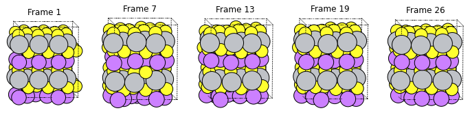
It looks like the Li atom is diffusing to the correct place, but it is easiest to visualize in AMSmovie:
!amsmovie "{m3gnet_rb_job.results.rkfpath()}"
Conclusion: We have reasonable reaction boost settings for M3GNet-UP-2022. This does not guarantee that the settings will be appropriate with the retrained model (for example because we expect the barrier to be higher), but it is likely to work.
Run simple active learning using ReactionBoost MD
al_s = plams.Settings()
al_s.input.ams.ActiveLearning.SuccessCriteria.Energy.Relative = 0.0012
al_s.input.ams.ActiveLearning.SuccessCriteria.Forces.MaxDeviationForZeroForce = 0.25
al_s.input.ams.ActiveLearning.Steps.Type = "Linear"
al_s.input.ams.ActiveLearning.Steps.Linear.Start = 15
al_s.input.ams.ActiveLearning.Steps.Linear.StepSize = 50
al_s.input.ams.ActiveLearning.InitialReferenceData.Load.Directory = (
    prelim_al_job2.results.get_reference_data_directory()
)
al_s.input.ams.ActiveLearning.InitialReferenceData.Load.FromPreviousModel = "No"


ml_s = plams.Settings()
ml_s.input.ams.MachineLearning.Backend = "M3GNet"
ml_s.input.ams.MachineLearning.LoadModel = (
    prelim_al_job2.results.get_params_results_directory()
)
ml_s.input.ams.MachineLearning.MaxEpochs = 200
ml_s.input.ams.MachineLearning.Target.Forces.MAE = 0.03
sal_job = SimpleActiveLearningJob(
    name="sal_lidiffusion_rb",
    settings=al_s + dft_s + ml_s + rb_s,
    molecule={"": defective_1, "final": defective_2},
)
print(sal_job.get_input())
ActiveLearning
  InitialReferenceData
    Load
      Directory /path/to/plams_workdir.007/al_defective/step7_attempt1_reference_data
      FromPreviousModel False
... output trimmed ....
         0.0000000000    11.9106205833     0.0000000000
         0.0000000000     0.0000000000    12.3498100000
  End
End
# plams.config.jobmanager.hashing = None
sal_job.run(watch=True);
[25.03|13:06:03] JOB sal_lidiffusion_rb STARTED
[25.03|13:06:03] Renaming job sal_lidiffusion_rb to sal_lidiffusion_rb.002
[25.03|13:06:03] JOB sal_lidiffusion_rb.002 RUNNING
[25.03|13:06:04] Simple Active Learning 2024.101,  Nodes: 1, Procs: 8
[25.03|13:06:06] Composition of main system: Li23S48Ti24
... output trimmed ....
[25.03|15:25:14] Rerunning the simulation with the final parameters...
[25.03|15:25:37] Copying final_production_simulation/ams.rkf to ams.rkf
[25.03|15:25:37] Goodbye!
[25.03|15:25:37] JOB sal_lidiffusion_rb.002 FINISHED
[25.03|15:25:37] JOB sal_lidiffusion_rb.002 SUCCESSFUL
m3gnet_new_s = sal_job.results.get_production_engine_settings()
m3gnet_new_s = prelim_al_job2.results.get_production_engine_settings()
Run NEB with retrained M3GNet
# constraint_s = plams.Settings()
# constraint_s.input.ams.Constraints.Atom = 8
defective_1_perturbed = defective_1.copy()
defective_1_perturbed.perturb_atoms()
defective_2_perturbed = defective_2.copy()
defective_2_perturbed.perturb_atoms()
m3gnet_new_neb_job = plams.AMSJob(
    settings=m3gnet_new_s + neb_s,  # + constraint_s,
    molecule={"": defective_1, "final": defective_2},
    name="m3gnet_new_neb",
)
m3gnet_new_neb_job.run();
[25.03|15:25:37] JOB m3gnet_new_neb STARTED
[25.03|15:25:37] JOB m3gnet_new_neb RUNNING
[25.03|15:25:58] JOB m3gnet_new_neb FINISHED
[25.03|15:25:58] JOB m3gnet_new_neb SUCCESSFUL
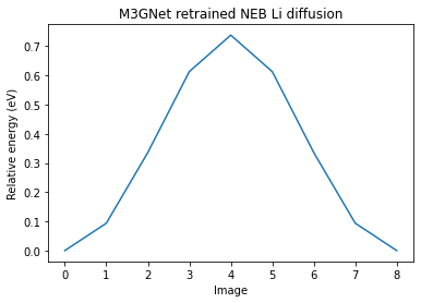
m3gnet_new_res = m3gnet_new_neb_job.results.get_neb_results(unit="eV")
print(f"Left barrier: {m3gnet_new_res['LeftBarrier']:.3f} eV")
print(f"Right barrier: {m3gnet_new_res['RightBarrier']:.3f} eV")
Left barrier: 0.738 eV
Right barrier: 0.738 eV
# ref_results = [0.0, 0.144, 0.482, 0.816, 0.963, 0.816, 0.482, 0.144, 0.0]  # from Quantum ESPRESSO DFT calculation
nImages = m3gnet_new_res["nImages"]
relative_energies = np.array(m3gnet_new_res["Energies"]) - m3gnet_new_res["Energies"][0]
plt.plot(relative_energies)
plt.xlabel("Image")
plt.ylabel("Relative energy (eV)")
plt.title("M3GNet retrained NEB Li diffusion");
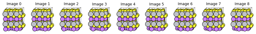
fig, axes = plt.subplots(1, len(m3gnet_new_res["Molecules"]), figsize=(15, 5))

for i, mol in enumerate(m3gnet_new_res["Molecules"]):
    plams.plot_molecule(mol, ax=axes[i], rotation="-85x,-5y,0z")
    axes[i].set_title(f"Image {i}")
Let’s run DFT calculations on these frames to compare. We can do this using the “Replay” task.
Note: The DFT calculations may take a few minutes to complete.
replay_s = plams.Settings()
replay_s.input.ams.Task = "Replay"
replay_s.input.ams.Replay.File = os.path.abspath(m3gnet_new_neb_job.results.rkfpath())
replay_s.input.ams.Properties.Gradients = "Yes"

replay_dft_job = plams.AMSJob(
    settings=replay_s + dft_s, name="replay_m3gnet_new_neb_with_dft"
)
replay_dft_job.run(watch=True);
[25.03|15:26:03] JOB replay_m3gnet_new_neb_with_dft STARTED
[25.03|15:26:03] JOB replay_m3gnet_new_neb_with_dft RUNNING
[25.03|15:26:03] replay_m3gnet_new_neb_with_dft: AMS 2024.101  RunTime: Mar25-2024 15:26:03  ShM Nodes: 1  Procs: 1
[25.03|15:26:03] replay_m3gnet_new_neb_with_dft: Starting trajectory replay ...
[25.03|15:26:03] replay_m3gnet_new_neb_with_dft: Replaying frame #1/9 (#320 in original trajectory)
... output trimmed ....
[25.03|15:38:47] replay_m3gnet_new_neb_with_dft: Trajectory replay complete.
[25.03|15:38:47] replay_m3gnet_new_neb_with_dft: Number of QE evaluations: 9
[25.03|15:38:47] replay_m3gnet_new_neb_with_dft: NORMAL TERMINATION
[25.03|15:38:47] JOB replay_m3gnet_new_neb_with_dft FINISHED
[25.03|15:38:47] JOB replay_m3gnet_new_neb_with_dft SUCCESSFUL
When using “Replay” on a NEB job, the results are stored in the normal NEB format. Thus we can use the .get_neb_results() method also on this job:
dft_energies = replay_dft_job.results.get_neb_results(unit="eV")["Energies"]
dft_relative_energies = np.array(dft_energies) - dft_energies[0]
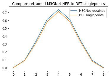
plt.plot(relative_energies)
plt.plot(dft_relative_energies)
plt.legend(["M3GNet retrained", "DFT singlepoints"])
plt.title("Compare retrained M3GNet NEB to DFT singlepoints");
See also
Python Script
#!/usr/bin/env python
# coding: utf-8

# ## Initialization

import scm.plams as plams
import os
import numpy as np
import matplotlib.pyplot as plt
import scm.params as params
from scm.simple_active_learning import SimpleActiveLearningJob


plams.init()


# ## Create structures
#
# ### Create primitive cell from coordinates

# for plotting in Jupyter notebooks
rotation = "-85x,-5y,0z"

# create structure
primitive = plams.AMSJob.from_input(
    """
    System
        Atoms
            Li 0. 0. 0.
            Ti 0. 0. 3.087452499999999
            S 0. 1.985103430533333 4.551328274799999
            S 1.71915 0.9925517153000001 1.6235767252
        End
        Lattice
            3.4383 0.0 0.0
            -1.71915 2.977655145833333 0.0
            0.0 0.0 6.174905
        End
    End
"""
).molecule[""]
plams.plot_molecule(primitive, rotation=rotation)


# ### Create a supercell.
#
# Here we a reasonably-sized supercell.  If the cell is very small, it is actually quite inefficient for training the machine learning potential. If every atom sees its own periodic image then there will not be sufficient variety in the atomic environments for the ML potential to be able to extrapolate to unseen environments. **It is recommended to use a larger supercell**.

supercell = primitive.supercell([[3, 0, 0], [2, 4, 0], [0, 0, 2]])
for at in supercell:
    at.properties = plams.Settings()
plams.plot_molecule(supercell, rotation=rotation)


print("Lattice vectors")
print(supercell.lattice)
print(f"Number of atoms: {len(supercell)}")


# ### Create Li vacancy in two different places

li_indices = [i for i, at in enumerate(supercell, 1) if at.symbol == "Li"]
print(f"Li indices (starting with 1): {li_indices}")


# Pick the first Li atom, and get its nearest Li neighbor.
#
# Note that the PLAMS distance_to function ignores periodic boundary conditions, which in this case is quite convenient as it will make the visualization easier if the Li atom diffuses inside the unit cell and doesn't cross the periodic boundary.

first_index = li_indices[0]
li1 = supercell[first_index]
li1.properties.region = "DiffusingLi"
distances = [li1.distance_to(supercell[x]) for x in li_indices[1:]]
nearest_neighbor_index = li_indices[np.argmin(distances) + 1]
li2 = supercell[nearest_neighbor_index]
target_coords = li2.coords
print(f"First Li atom: {li1}")
print(f"Second Li atom: {li2}")


# The goal is to make a Li atom diffuse between these two positions.
#
# For this, we will first delete the second Li atom, and then create a new structure in which the first Li atom is translated to the second Li atom coordinates.

defective_1 = supercell.copy()
defective_1.delete_atom(defective_1[nearest_neighbor_index])
defective_2 = supercell.copy()
defective_2.delete_atom(defective_2[nearest_neighbor_index])
defective_2[first_index].coords = li2.coords


plams.plot_molecule(defective_1, rotation=rotation)
plt.title("Initial structure")
plt.gcf().savefig("picture1.png")
plt.clf()


# The Li atom in the bottom left corner will diffuse to the right (the vacancy will diffuse to the left):

plams.plot_molecule(defective_2, rotation=rotation)
plt.title("Final structure")
plt.gcf().savefig("picture2.png")
plt.clf()


# ## Initial validation of diffusion barrier with NEB and M3GNet-UP-2022
#
# ### M3GNet-UP-2022 NEB job

m3gnet_up_s = plams.Settings()
m3gnet_up_s.input.MLPotential.Model = "M3GNet-UP-2022"

neb_s = plams.Settings()
neb_s.input.ams.Task = "NEB"
neb_s.input.ams.NEB.PreoptimizeWithIDPP = "Yes"
neb_s.input.ams.NEB.Images = 7


m3gnet_up_neb_job = plams.AMSJob(
    settings=m3gnet_up_s + neb_s,
    molecule={"": defective_1, "final": defective_2},
    name="m3gnet_up_neb",
)
m3gnet_up_neb_job.run()
# ### M3GNet-UP-2022 NEB results

m3gnet_up_res = m3gnet_up_neb_job.results.get_neb_results(unit="eV")
print(f"Left barrier: {m3gnet_up_res['LeftBarrier']:.3f} eV")
print(f"Right barrier: {m3gnet_up_res['RightBarrier']:.3f} eV")


# ref_results = [0.0, 0.144, 0.482, 0.816, 0.963, 0.816, 0.482, 0.144, 0.0]  # from Quantum ESPRESSO DFT calculation
nImages = m3gnet_up_res["nImages"]
relative_energies = np.array(m3gnet_up_res["Energies"]) - m3gnet_up_res["Energies"][0]
plt.plot(relative_energies)
plt.xlabel("Image")
plt.ylabel("Relative energy (eV)")
plt.title("M3GNet-UP-2022 NEB Li diffusion")
plt.gcf().savefig("picture3.png")
plt.clf()


fig, axes = plt.subplots(1, len(m3gnet_up_res["Molecules"]), figsize=(15, 5))

for i, mol in enumerate(m3gnet_up_res["Molecules"]):
    plams.plot_molecule(mol, ax=axes[i], rotation=rotation)
    axes[i].set_title(f"Image {i}")


# get_ipython().system('amsmovie "{m3gnet_up_neb_job.results.rkfpath()}"')


# ## DFT reference engine settings
#
# Are the above M3GNet-UP-2022 results any good? Let's compare to DFT calculations using the AMS "Replay" task.
#
# "Replay" is just a series of singlepoints on the previous NEB structures. It is not a NEB calculation.
#
# Here we use the Quantum ESPRESSO engine available in AMS2024.

dft_s = plams.Settings()
dft_s.input.QuantumESPRESSO.System.occupations = "Smearing"
dft_s.input.QuantumESPRESSO.System.degauss = 0.005
# for production purposes always manually check that ecutwfc and ecutrho are high enough
# here we set a fairly low ecutwfc to speed up the calculation
dft_s.input.QuantumESPRESSO.System.ecutwfc = 30.0
dft_s.input.QuantumESPRESSO.System.ecutrho = 240.0
# decrease mixing_beta for more robust SCF convergence
dft_s.input.QuantumESPRESSO.Electrons.mixing_beta = 0.3
dft_s.input.QuantumESPRESSO.Electrons.conv_thr = 1.0e-5 * len(supercell)
# for a small cell one should ideally use more k-points than just the gamma point
# by settings K_Points._h = "gamma" we use the faster gamma-point-only
# implementation in Quantum ESPRESSO
dft_s.input.QuantumESPRESSO.K_Points._h = "gamma"
# SCM_DISABLE_MPI launches ams in serial, but will still run Quantum ESPRESSO in parallel
dft_s.runscript.preamble_lines = ["export SCM_DISABLE_MPI=1"]


# ## Run DFT calculations on the NEB points from M3GNet-UP-2022
#
# Note: The DFT calculations may take a few minutes to complete.

replay_s = plams.Settings()
replay_s.input.ams.Task = "Replay"
replay_s.input.ams.Replay.File = os.path.abspath(m3gnet_up_neb_job.results.rkfpath())
replay_s.input.ams.Properties.Gradients = "Yes"

replay_dft_job = plams.AMSJob(settings=replay_s + dft_s, name="replay_m3gnet_up_neb_with_dft")
replay_dft_job.run(watch=True)
# When using "Replay" on a NEB job, the results are stored in the normal NEB format. Thus we can use the ``.get_neb_results()`` method also on this job:

dft_energies = replay_dft_job.results.get_neb_results(unit="eV")["Energies"]
dft_relative_energies = np.array(dft_energies) - dft_energies[0]

plt.plot(relative_energies)
plt.plot(dft_relative_energies)
plt.legend(["M3GNet-UP-2022", "DFT singlepoints"])
plt.title("Compare M3GNet-UP-2022 NEB to DFT singlepoints")
plt.gcf().savefig("picture4.png")
plt.clf()


# **Conclusion**: M3GNet-UP-2022 significantly underestimates the diffusion barrier compared to DFT calculations. **This motivates the reparametrization**

# ## Store DFT results for later
#
# Since we already performed some DFT calculations, we may as well add them to the training set.

ri = params.ResultsImporter(settings={"units": {"energy": "eV", "forces": "eV/angstrom"}})
ri.add_trajectory_singlepoints(
    replay_dft_job,
    properties=["energy", "forces"],
    indices=[0, 1, 2, 3, 4],
    data_set="training_set",
)
ri.add_trajectory_singlepoints(
    replay_dft_job,
    properties=["energy", "forces"],
    indices=[5],
    data_set="validation_set",
)
yaml_dir = "lidiffusion_initial_reference_data"
ri.store(yaml_dir, backup=False)


# ## Preliminary active learning jobs with equilibrium MD
#
# Let's first run some simple NVT MD with active learning for both the
# * stochiometric system (``supercell``), and
# * defective system (``defective_1``)
#
# This is just to get a good general sampling before setting up the reaction boost to explicitly sample the diffusion process.

# ### Active Learning for stoichiometric system
#
# The stoichiometric system is a perfect crystal with not so many atoms. The forces will be very close to 0 also after a few MD frames. However, even if the ML model predicts forces close to 0, the R^2 between predicted and reference forces may be quite low.
#
# In a case like this, it is reasonable to either
#
# * decrease the MinR2 success criterion, and/or
# * perturb the atomic coordinates of the initial structure a bit, so that the forces aren't extremely small
#
# Here, we do both of these:

nvt_md_s = plams.AMSNVTJob(nsteps=5000, timestep=0.5, temperature=400, tau=50, thermostat="Berendsen").settings

prelim_al_s = plams.Settings()
prelim_al_s.input.ams.ActiveLearning.InitialReferenceData.Load.Directory = os.path.abspath(yaml_dir)
prelim_al_s.input.ams.ActiveLearning.Steps.Type = "Geometric"
prelim_al_s.input.ams.ActiveLearning.Steps.Geometric.NumSteps = 7
prelim_al_s.input.ams.ActiveLearning.SuccessCriteria.Forces.MinR2 = 0.5
prelim_al_s.input.ams.ActiveLearning.AtEnd.RerunSimulation = "No"

ml_s = plams.Settings()
ml_s.input.ams.MachineLearning.Backend = "M3GNet"
ml_s.input.ams.MachineLearning.M3GNet.Model = "UniversalPotential"
ml_s.input.ams.MachineLearning.MaxEpochs = 100
ml_s.input.ams.MachineLearning.Target.Forces.MAE = 0.04

perturbed_supercell = supercell.copy()
perturbed_supercell.perturb_atoms(0.1)

prelim_al_job = SimpleActiveLearningJob(
    name="al_supercell",
    molecule=perturbed_supercell,
    settings=prelim_al_s + ml_s + nvt_md_s + dft_s,
)
prelim_al_job.run(watch=True)
# ### Active learning for defective system

prelim_al_s2 = prelim_al_s.copy()
prelim_al_s2.input.ams.ActiveLearning.InitialReferenceData.Load.Directory = (
    prelim_al_job.results.get_reference_data_directory()
)
prelim_al_s2.input.ams.ActiveLearning.InitialReferenceData.Load.FromPreviousModel = "No"
prelim_al_s2.input.ams.ActiveLearning.SuccessCriteria.Forces.MaxDeviationForZeroForce = 0.35

ml_s2 = plams.Settings()
ml_s2.input.ams.MachineLearning.Backend = "M3GNet"
ml_s2.input.ams.MachineLearning.LoadModel = prelim_al_job.results.get_params_results_directory()
ml_s2.input.ams.MachineLearning.MaxEpochs = 200
ml_s2.input.ams.MachineLearning.Target.Forces.MAE = 0.03

prelim_al_job2 = SimpleActiveLearningJob(
    name="al_defective",
    molecule=defective_1,
    settings=prelim_al_s2 + ml_s2 + nvt_md_s + dft_s,
)
prelim_al_job2.run(watch=True)
# ## Set up ReactionBoost MD simulation with M3GNet-UP-2022
#
# ReactionBoost simulations can be a bit tricky to set up.
#
# Before using ReactionBoost inside the Active Learning, it is best to verify that the simulation behaves reasonably when using M3GNet-UP-2022.
#
# So let's just run a normal ReactionBoost simulation with M3GNet-UP-2022:

md_s = plams.Settings()
md_s.Thermostat.Temperature = 300
md_s.Thermostat.Type = "Berendsen"
md_s.Thermostat.Tau = 5
md_s.InitialVelocities.Type = "Random"
md_s.InitialVelocities.Temperature = 300
md_s.ReactionBoost.Type = "RMSD"
md_s.ReactionBoost.NSteps = 480
md_s.ReactionBoost.Region = "DiffusingLi"
md_s.ReactionBoost.TargetSystem = "final"
md_s.ReactionBoost.RMSDRestraint.Type = "Harmonic"
md_s.ReactionBoost.RMSDRestraint.Harmonic.ForceConstant = 0.1
md_s.NSteps = 500
md_s.TimeStep = 0.5
md_s.Trajectory.SamplingFreq = 20
rb_s = plams.Settings()
rb_s.input.ams.Task = "MolecularDynamics"
rb_s.input.ams.MolecularDynamics = md_s


m3gnet_rb_job = plams.AMSJob(
    settings=m3gnet_up_s + rb_s,
    name="m3gnet_up_rb",
    molecule={"": defective_1, "final": defective_2},
)
m3gnet_rb_job.run()
N = 5  # show 5 structures
fig, axes = plt.subplots(1, N, figsize=(12, 5))
nEntries = m3gnet_rb_job.results.readrkf("History", "nEntries")
print(f"There are {nEntries} frames in the trajectory")
ind = np.linspace(1, nEntries, N, endpoint=True, dtype=np.int64)
for ax, i_frame in zip(axes, ind):
    plams.plot_molecule(
        m3gnet_rb_job.results.get_history_molecule(i_frame),
        ax=ax,
        rotation="-85x,5y,0z",
    )
    ax.set_title(f"Frame {i_frame}")


# It looks like the Li atom is diffusing to the correct place, but it is easiest to visualize in AMSmovie:

# get_ipython().system('amsmovie "{m3gnet_rb_job.results.rkfpath()}"')


# **Conclusion**: We have reasonable reaction boost settings for M3GNet-UP-2022. This does not guarantee that the settings will be appropriate with the retrained model (for example because we expect the barrier to be higher), but it is likely to work.

# ## Run simple active learning using ReactionBoost MD

al_s = plams.Settings()
al_s.input.ams.ActiveLearning.SuccessCriteria.Energy.Relative = 0.0012
al_s.input.ams.ActiveLearning.SuccessCriteria.Forces.MaxDeviationForZeroForce = 0.25
al_s.input.ams.ActiveLearning.Steps.Type = "Linear"
al_s.input.ams.ActiveLearning.Steps.Linear.Start = 15
al_s.input.ams.ActiveLearning.Steps.Linear.StepSize = 50
al_s.input.ams.ActiveLearning.InitialReferenceData.Load.Directory = (
    prelim_al_job2.results.get_reference_data_directory()
)
al_s.input.ams.ActiveLearning.InitialReferenceData.Load.FromPreviousModel = "No"


ml_s = plams.Settings()
ml_s.input.ams.MachineLearning.Backend = "M3GNet"
ml_s.input.ams.MachineLearning.LoadModel = prelim_al_job2.results.get_params_results_directory()
ml_s.input.ams.MachineLearning.MaxEpochs = 200
ml_s.input.ams.MachineLearning.Target.Forces.MAE = 0.03


sal_job = SimpleActiveLearningJob(
    name="sal_lidiffusion_rb",
    settings=al_s + dft_s + ml_s + rb_s,
    molecule={"": defective_1, "final": defective_2},
)
print(sal_job.get_input())


# plams.config.jobmanager.hashing = None
sal_job.run(watch=True)
m3gnet_new_s = sal_job.results.get_production_engine_settings()
m3gnet_new_s = prelim_al_job2.results.get_production_engine_settings()


# ## Run NEB with retrained M3GNet

# constraint_s = plams.Settings()
# constraint_s.input.ams.Constraints.Atom = 8
defective_1_perturbed = defective_1.copy()
defective_1_perturbed.perturb_atoms()
defective_2_perturbed = defective_2.copy()
defective_2_perturbed.perturb_atoms()
m3gnet_new_neb_job = plams.AMSJob(
    settings=m3gnet_new_s + neb_s,  # + constraint_s,
    molecule={"": defective_1, "final": defective_2},
    name="m3gnet_new_neb",
)
m3gnet_new_neb_job.run()
m3gnet_new_res = m3gnet_new_neb_job.results.get_neb_results(unit="eV")
print(f"Left barrier: {m3gnet_new_res['LeftBarrier']:.3f} eV")
print(f"Right barrier: {m3gnet_new_res['RightBarrier']:.3f} eV")


# ref_results = [0.0, 0.144, 0.482, 0.816, 0.963, 0.816, 0.482, 0.144, 0.0]  # from Quantum ESPRESSO DFT calculation
nImages = m3gnet_new_res["nImages"]
relative_energies = np.array(m3gnet_new_res["Energies"]) - m3gnet_new_res["Energies"][0]
plt.plot(relative_energies)
plt.xlabel("Image")
plt.ylabel("Relative energy (eV)")
plt.title("M3GNet retrained NEB Li diffusion")
plt.gcf().savefig("picture5.png")
plt.clf()


fig, axes = plt.subplots(1, len(m3gnet_new_res["Molecules"]), figsize=(15, 5))

for i, mol in enumerate(m3gnet_new_res["Molecules"]):
    plams.plot_molecule(mol, ax=axes[i], rotation="-85x,-5y,0z")
    axes[i].set_title(f"Image {i}")


# Let's run DFT calculations on these frames to compare. We can do this using the "Replay" task.
#
# Note: The DFT calculations may take a few minutes to complete.

replay_s = plams.Settings()
replay_s.input.ams.Task = "Replay"
replay_s.input.ams.Replay.File = os.path.abspath(m3gnet_new_neb_job.results.rkfpath())
replay_s.input.ams.Properties.Gradients = "Yes"

replay_dft_job = plams.AMSJob(settings=replay_s + dft_s, name="replay_m3gnet_new_neb_with_dft")
replay_dft_job.run(watch=True)
# When using "Replay" on a NEB job, the results are stored in the normal NEB format. Thus we can use the ``.get_neb_results()`` method also on this job:

dft_energies = replay_dft_job.results.get_neb_results(unit="eV")["Energies"]
dft_relative_energies = np.array(dft_energies) - dft_energies[0]

plt.plot(relative_energies)
plt.plot(dft_relative_energies)
plt.legend(["M3GNet retrained", "DFT singlepoints"])
plt.title("Compare retrained M3GNet NEB to DFT singlepoints")
plt.gcf().savefig("picture6.png")
plt.clf()