Simple (MD) Active Learning
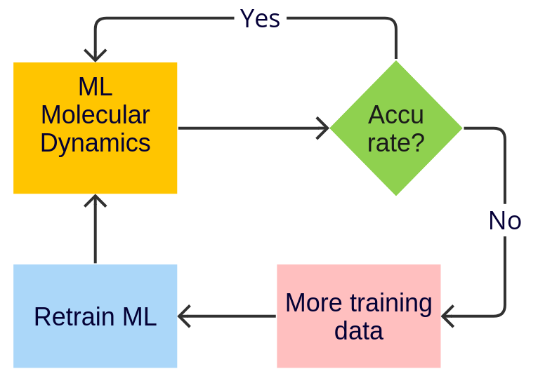
Starting with AMS2024, the Amsterdam Modeling Suite contains a Simple (MD) Active Learning workflow for on-the-fly training of machine learning potentials during molecular dynamics (MD).
In this tutorial, you will
apply transfer learning techniques to “fine-tune” the M3GNet Universal Potential (M3GNet-UP-2022) to make it more accurate for a given system
generate all training and validation data on-the-fly during an MD simulation
To run the Simple Active Learning workflow, you need a license for Advanced Workflows and Tools, Classical force fields and machine learning potentials, and the reference engine.
Important
Make sure that M3GNet is installed correctly.
Prerequisite: Follow the M3GNet: Universal ML Potential tutorial.
Approximate tutorial running time:
On CPU: 30 minutes
On GPU: 15 minutes
(The speedup on the GPU becomes much more significant if you have larger molecules/systems)
Initial setup
 → MD Active Learning
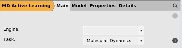
An active learning run has 5 required types of input:
Initial structure
Reference engine settings
Molecular dynamics settings
Machine learning model (e.g., M3GNet) settings
Active learning settings
Here we go through them in sequence:
Initial structure
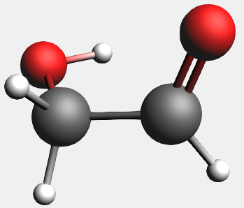
To get the initial structure, you can either draw a molecule, find it in the search bar, import the coordinates from a .xyz file or import from SMILES.
OCC=O and click OKFeel free to use a different molecule if you prefer.
Important
1. Make sure that the initial structure is “reasonable”. It doesn’t have to be geometry-optimized (in fact it is good if not all forces are exactly 0), but if the forces are very high then the temperature will rise very quickly in the MD simulation.
2. Make sure that your reference engine can reliably calculate energies and forces for your system. For example, make sure that the SCF converges in DFT calculations. This is easiest to check by running a few normal DFT calculations before using the active learning.
Reference engine settings
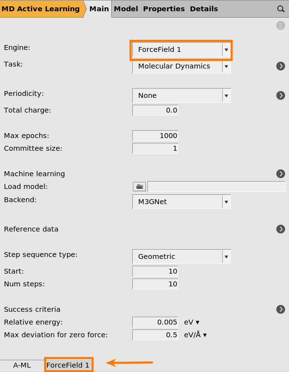
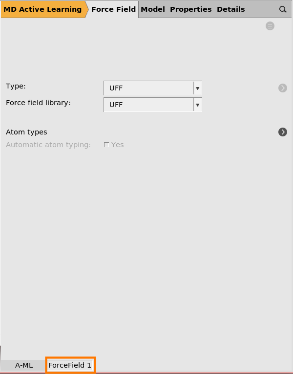
This will use UFF as the reference engine. In this tutorial we will use the UFF force field as it is very fast to evaluate and is included with all AMS licenses.
If you have a license to run a different compute engine like ADF or DFTB, feel free to select that engine instead, and set any engine settings like basis set on the corresponding panel at the bottom of the window.
Note
UFF can give very strange results for heavily distorted molecules that may form during the active learning.
So use a different reference engine if you can!
Molecular dynamics settings
 button next to Task: MolecularDynamics
100000.5 fs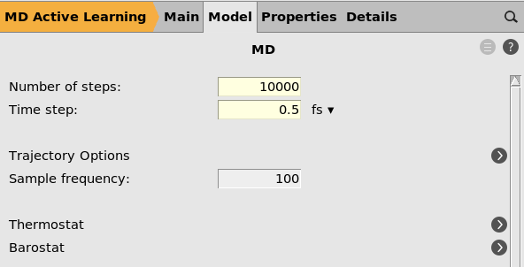 button next to Thermostat
NHC300 K200 fs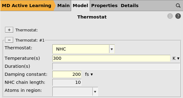
Tip
You may consider setting the damping constant to a much smaller value, for
example 10 fs.
This will cool down the system more quickly in case the temperature starts to rise uncontrollably, which may happen
if the initial structure is very far from a minimum, or
when the MD simulation explores configuration space that the ML model has not seen before
Machine learning model settings
2001 (default)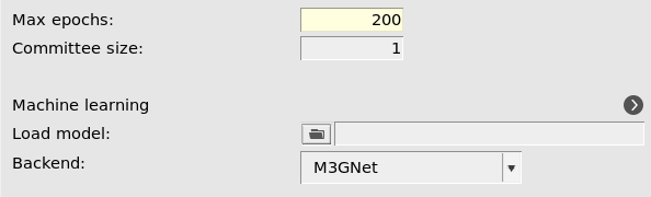 button next to Machine learning
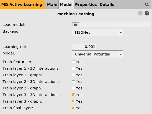
This will start the parametrization from the M3GNet-UP-2022 parameters. You can also train a custom M3GNet model completely from scratch by setting Model → Custom.
However, in this tutorial we will fine-tune the Universal Potential, so make sure that Model is set to Universal Potential.
You can also select which layers to retrain. Feel free to experiment with different combinations.
If you increase the Committee size you will train multiple models. This is typically not so useful when starting from the universal potential, since the models will become very similar. It also significantly increases the computational cost and memory requirements. For this reason, we only train a single model (committee size = 1) in this tutorial.
Tip
The Load model option lets you load a previously trained model.
For example,
you may have trained an initial M3GNet model using your own training data (not generated with active learning) in ParAMS, or
you wish to continue with a new active learning run for a different system, temperature, or other simulation settings.
Then you can specify the ParAMS results directory in the Load model
option. This directory should contain the subdirectories optimization
and settings_and_initial_data. It is typically called something like
step5_attempt4_training/results if you generated it using active
learning.
Active learning settings
Initial reference data
next to Reference data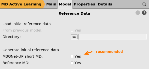
On the Reference data panel you can
choose to load reference data from a directory containing ParAMS .yaml files
Specify how to generate the initial reference data
If you do not specify anything on this panel, it is the same as ticking the Reference MD box.
Tip
If (and only if) the M3GNet universal potential produces reasonable results/structures for your kind of system, we recommend to tick the M3GNet-UP short MD option.
Feel free to choose one or the other.
For details, see the simple active learning documentation for initial reference data
Step sequence type
Geometric (default)10 (default)5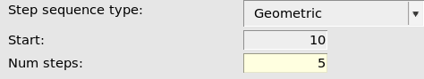
This will divide the MD simulation into 5 segments. The first segment is
10 MD frames. This means that after the first 10 MD frames, a reference
calculation will be performed on the current MD structure and the results compared
to the prediction.
If the results are
accurate enough, then the MD simulation continues
not accurate enough, then the model will be retrained
For details, see the simple active learning documentation for Step
Success criteria
button next to Success criteria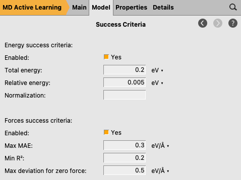
The success criteria determine how good the agreement needs to be between the reference calculation and prediction.
Feel free to experiment with different values. Here, we leave them all at the default values.
For details, see the documentation for success criteria
Reasonable simulation criteria
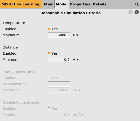
Here you can set a maximum allowed temperature and a minimum allowed interatomic distance. If these criteria are exceeded, all subsequent MD frames are discarded and the model will be retrained.
Hopefully these criteria are never exceeded! If they are, you may consider increasing the number of active learning steps to more frequently run reference calculations.
If you train a committee (not done in this tutorial), you can also set criteria for the maximum allowed uncertainty in the energy and forces predictions.
For details, see the documentation for reasonable simulation criteria
Other active learning settings
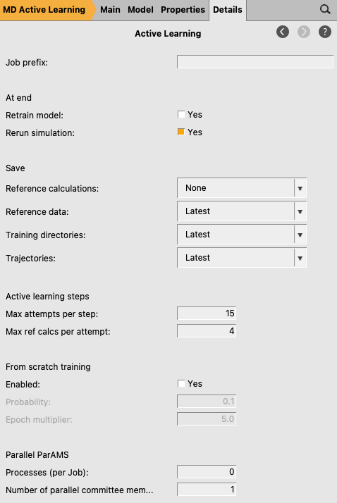
Here you can choose
Run the active learning job and view results
Then save and run the job:
Log file
The .log file is continually updated with information about the progress of the active learning, including
the current active learning step and attempt
results from the success criteria (reported on the lines
CheckEnergyandCheckForces)mean absolute error for energies and forces for training and validation sets after each retraining
timing information
The active learning loop is not deterministic, so your results are likely to look a little different. At the end of the job, the bottom of the log file may look like this:
Current (cumulative) timings:
                                          Time (s) Fraction
    Ref. calcs                               20.44    0.034
    ML training                             365.82    0.608
    Simulations                             215.21    0.358


Step 5 finished successfully!

--- Begin summary ---
Step  Attempt Status   Reason      finalframe_forces_max_delta
    1      1 FAILED   Inaccurate                  1.7423
    1      2 SUCCESS  Accurate                    0.5734
    2      1 FAILED   Inaccurate                  1.0679
    2      2 SUCCESS  Accurate                    0.3920
    3      1 FAILED   Inaccurate                  0.9762
    3      2 FAILED   Inaccurate                  0.7560
    3      3 SUCCESS  Accurate                    0.1781
    4      1 FAILED   Inaccurate                  0.3389
    4      2 SUCCESS  Accurate                    0.2827
    5      1 SUCCESS  Accurate                    0.5300
--- End summary ---

The engine settings for the final trained ML engine are:

Engine MLPotential
  Backend M3GNet
  MLDistanceUnit angstrom
  MLEnergyUnit eV
  Model Custom
  ParameterDir /path/step4_attempt1_training/results/optimization/m3gnet/m3gnet
EndEngine

Active learning finished!
Rerunning the simulation with the final parameters...
Goodbye!
In the timings, we see that very little time was spent on reference calculations, which makes sense since we used the UFF force field.
In the summary, some of the attempts are marked as FAILED. This means that the energy/forces of the structure in the MD simulation was not predicted accurately enough in comparison to the reference method. This triggers a retraining of the ML model, and then the step is reattempted.
The final engine settings contains an Engine block that can be used in AMS text input files to use your final trained model in production simulations. Note that the units are always “eV” and “angstrom”, no matter which units you use for the reference data in ParAMS.
Tip
You can copy-paste all the lines Engine MLPotential …
EndEngine directly into AMSinput, in order to set up a new job with
your trained model.
MD trajectory
You can view the current progress of the MD simulation in AMSmovie:
This opens the most recent trajectory file. Note that this file may be deleted as the active learning progresses. To open the most recent file, you may need to close AMSmovie and start it again.
Tip
In AMSMovie, you can select File → Related files to see some of the other available trajectory files.
Note
If you open the trajectory files before the active learning loop as finished, you may see strange jumps or discontinuities in the plotted Energy.
This is because the ML model is retrained on-the-fly!
If the “Rerun simulation at end” option is enabled (it is enabled by default),
then the trajectory in the final_production_simulation directory contains
the entire trajectory calculated with only the final parameters.
Training and validation results
You can view the results of the training in ParAMS:
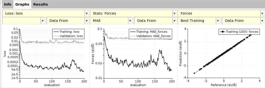
This lets you view the loss-function vs. epoch, scatter plots for predicted vs. reference forces, etc. For details on how to use ParAMS, see the ParAMS tutorials.
Note that the ParAMS results may be deleted as the active learning progresses. To open the most recent results, you may need to close ParAMS and start it again.
Note
Your results may be different from those shown here, as molecular dynamics simulation relies on random numbers for the initial velocities.
This opens up a new AMSinput window with the engine settings for the best trained model.
You can then use it to run any kind of production simulation.
Further reading
The Simple Active Learning Documentation contains a detailed description of all input options.
Learn how to set up active learning workflows in Python.
Check out the liquid water case study to see how to use active learning to exactly reproduce the liquid water self-diffusion coefficient, radial distribution functions, and density.