ACE Reaction Network
The Amsterdam Modeling Suite has several tools available to create reactions networks:
ACE reaction (this tutorial),
PES Exploration, and
Out of these, ACE reaction is the fastest tool, and can be used for quick initial guesses of a network.
ACE Reaction generates a reaction network from user-specified reactants and products. It creates initial guesses for intermediates based only on molecular graphs, and then confirms the validity of the intermediates using geometry optimization.
In this tutorial you will learn to use ACE reaction to generate a network, and interpret the results.
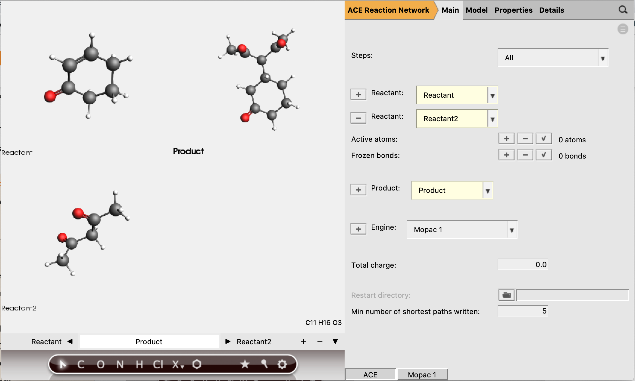
We will use the following addition reaction as our example.
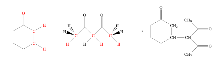
ACE reaction needs a selection of active atoms as input, and the set should never be larger than 11 atoms. The red atoms in the above figure are the atoms we expect to be involved in bond-breaking or forming.
We can use our chemical intuition to predict a reaction mechanism, and then see if ACE reaction indeed suggests this reaction as a likely option.
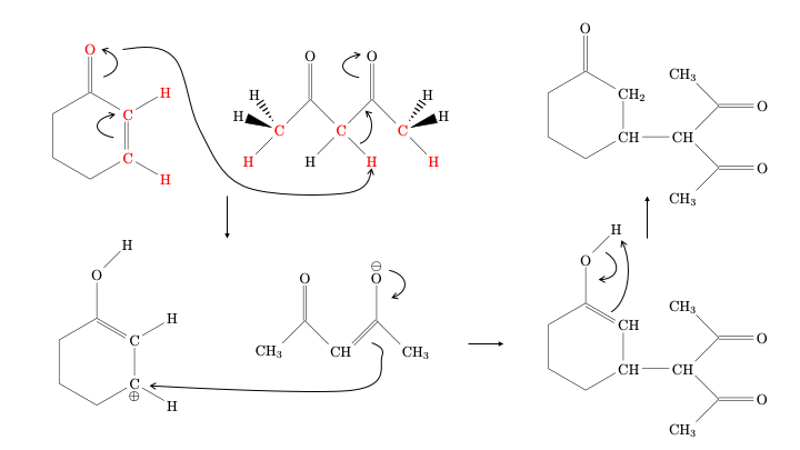
The expected reaction mechanism would involve
deprotonation of the diketone (the negative charge will be stabilized by conjugation with the two oxygen atoms), followed by
electrophilic addition to the protonated cyclohexenone molecule, and
finalized by a proton jump to recreate the ketone from the enol.
Set up the ACE reaction network computation
 →
→ 
Now the reactant and product structures can be either imported or drawn. In the drawing panel on the left of the window, the bar at the bottom shows that the reactant is selected and can now be created.
Tip
The SMILES strings for these molecules are:
Reactant 1:
O=C1C=CCCC1Reactant 2:
CC(=O)CC(C)=OProduct:
CC(=O)C(C(C)=O)C1CCCC(=O)C1
here and save and unpack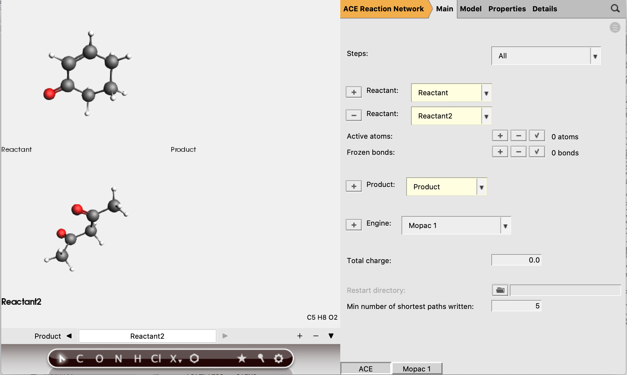
Reactant 1 should have 5 active atoms (2 H, 2 C, 1 O)
Reactant 2 should have 6 active atoms (3 H, 3 C)
Total number of active atoms: 11
See the figure below for the exact atoms to select:
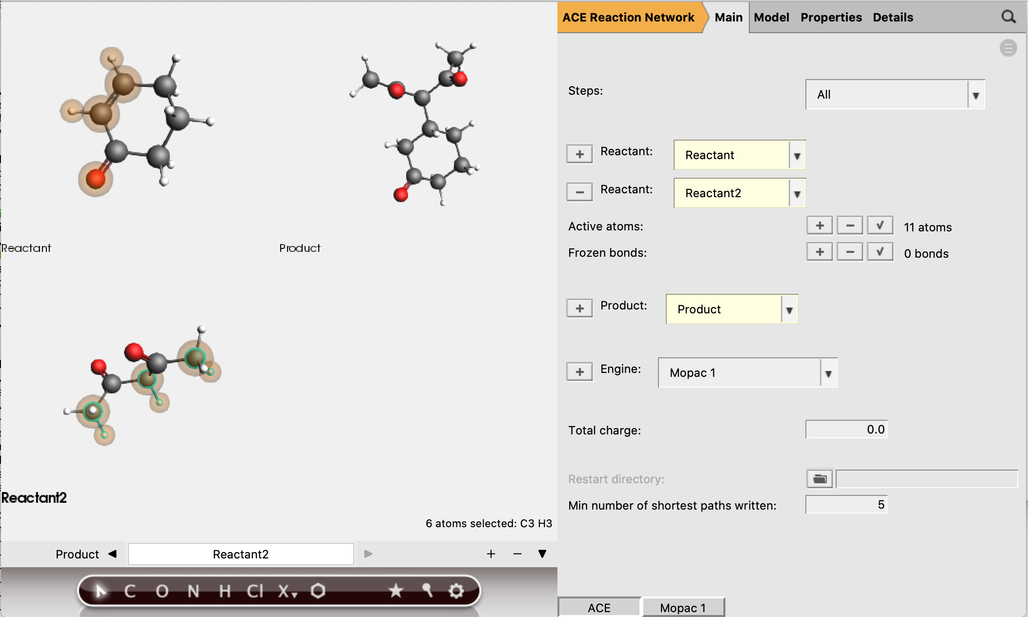
The active atoms are the only atoms allowed to be involved in bond-breaking and bond-forming processes.
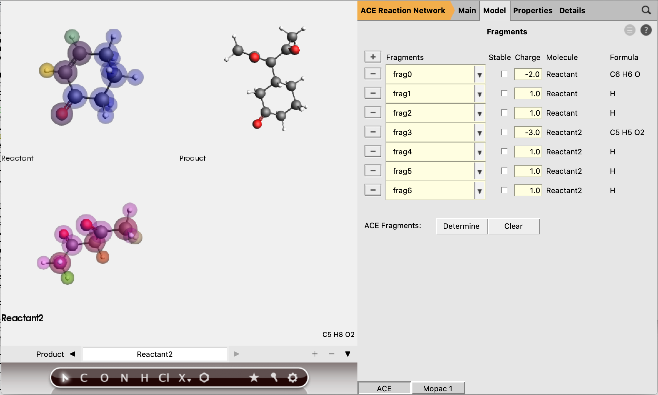
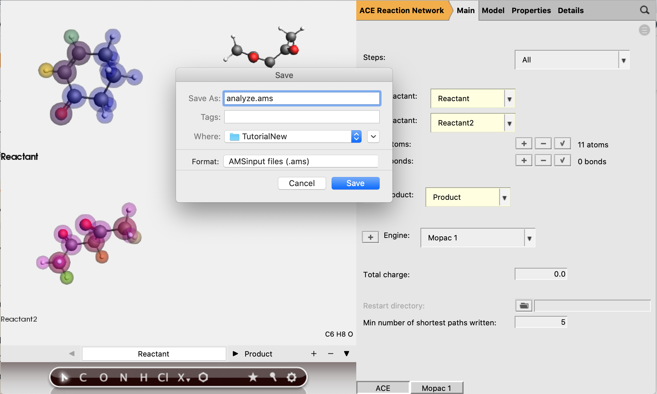
These fragments are the smallest possible fragment, based on the selection of active atoms. It is good practice to check the guessed fragment charges, to see if they will lead to the correct charges for any intermediate molecules we expect.
In this case, we can see that all the active H-atoms have a charge of +1, which is compensated by the fragments they are coordinated to.
The first step of our proposed reaction indeed involves a proton transfer, which requires the transferred H-atom to have a positive charge. Therefore the expected charges of the proposed intermediates match the guessed fragment charges, and we can accept them as reasonable guesses.
All fragments are estimated to be non-stable, which means that intermediates that contain a pure fragment as one of its submolecules will not be accepted.
We are now ready to run our ACE reaction job. An ACE reaction calculation always consists of three steps.
Intermediate generation by iteratively breaking and forming bonds in the reactant molecules.
Creating a reaction network by determining which pairs of newly created intermediates are connected by an elementary reaction.
Minimizing the reaction network by eliminating paths that involve to many bond-breaking and forming processes.
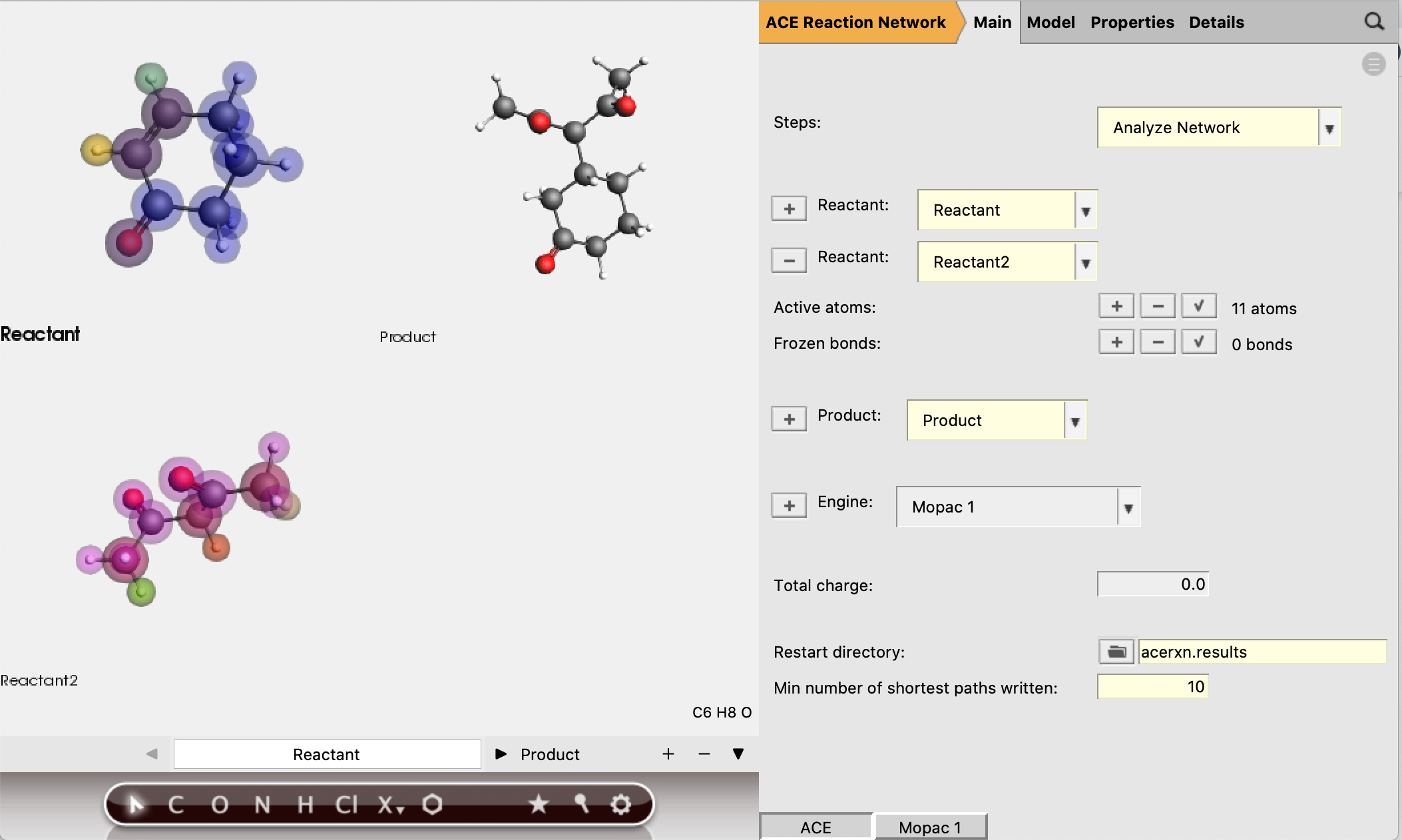
By default these three steps will all be performed, but the user also has the option to select only one of the steps. If only step 2 or 3 is selected, a restart directory needs to be provided. In this case we keep the default selection of All.
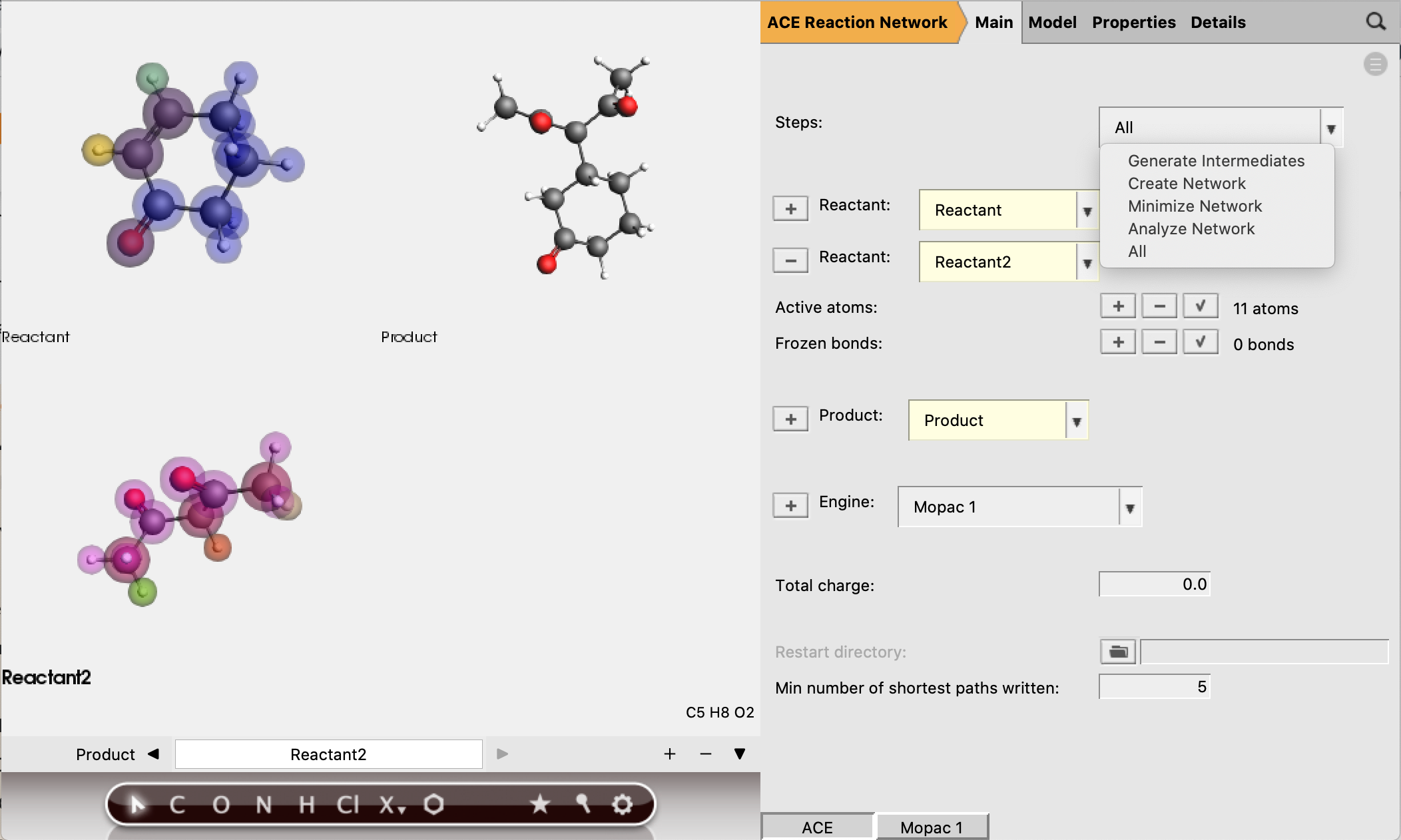
There is a final option Analyze Network, which also requires a restart directory to be specified. This option reads a network from the restart directory, and allows the ‘min number of shortest paths written’ (default is 5) to be adjusted. The selection of shortest paths will then be written to a separate RKF file. The setting ‘min number of shortest paths written’ can be found in the main panel.
Running an ACE reaction job
It will take a few minutes for the job to finish.
Note
ACE reaction jobs may not show in AMSjobs by default. You can make them visible by checking the option for Filter → Other.
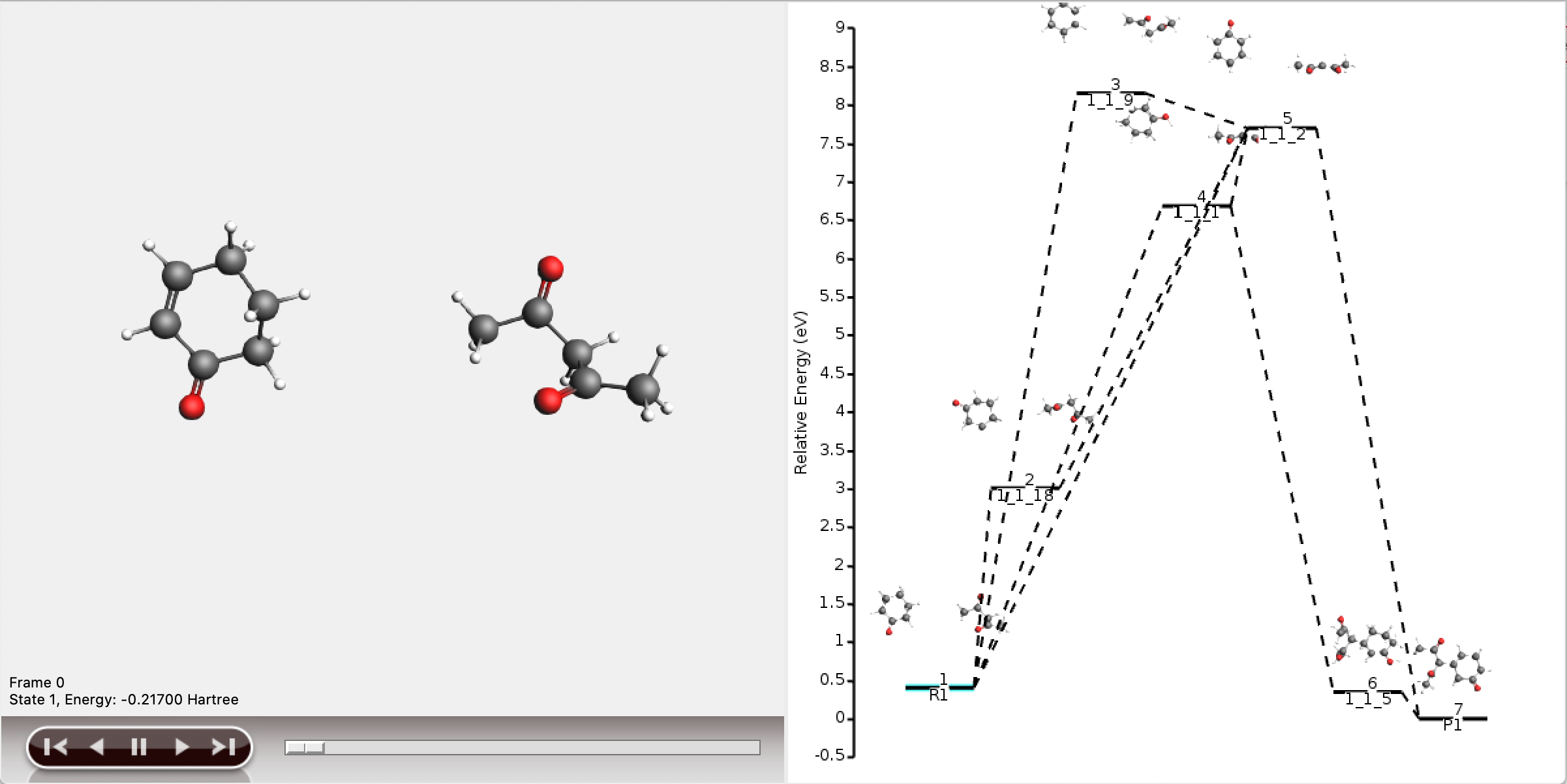
This will open the five shortest paths found from reactant to product.
It is also possible to view the full reaction network in AMSmovie, but this will be difficult to interpret.
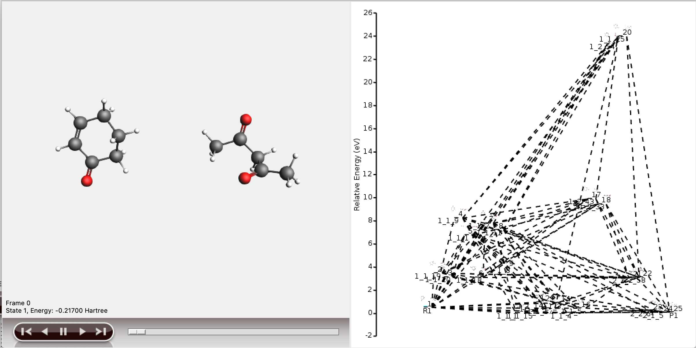
As can be seen, the full network contains too much information to display meaningfully in AMSmovie. We will use the shortest_paths window for any further interpretation.
Interpret an ACE reaction job
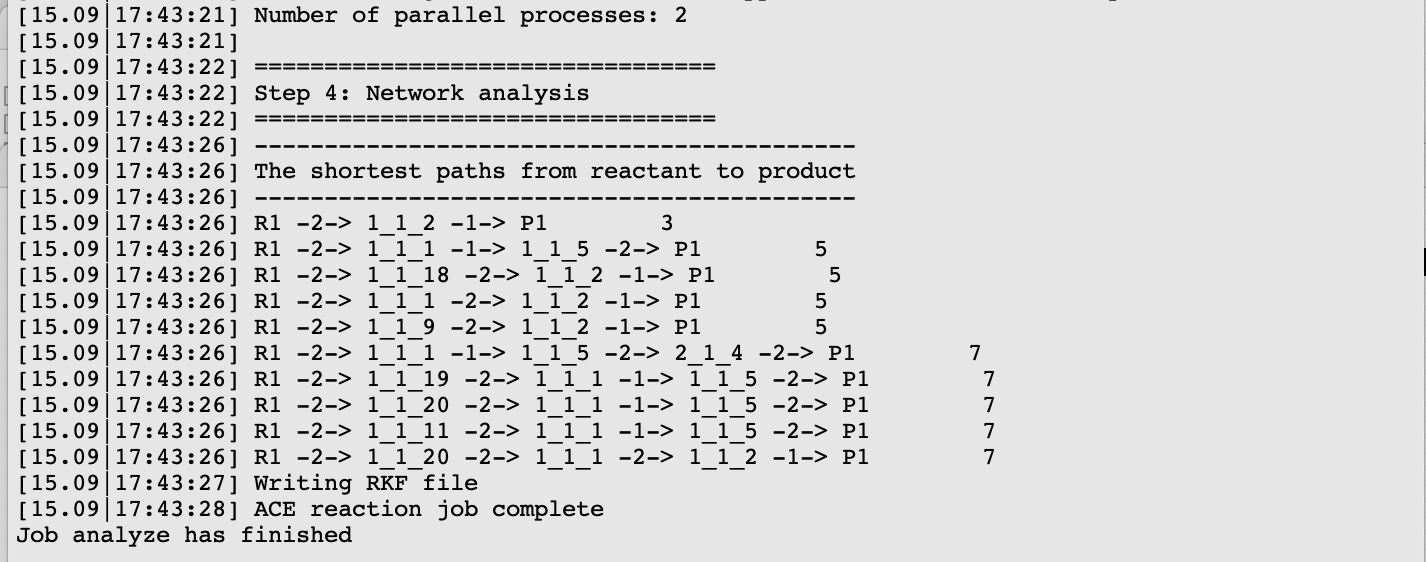
The five shortest paths are also displayed schematically in the logfile.
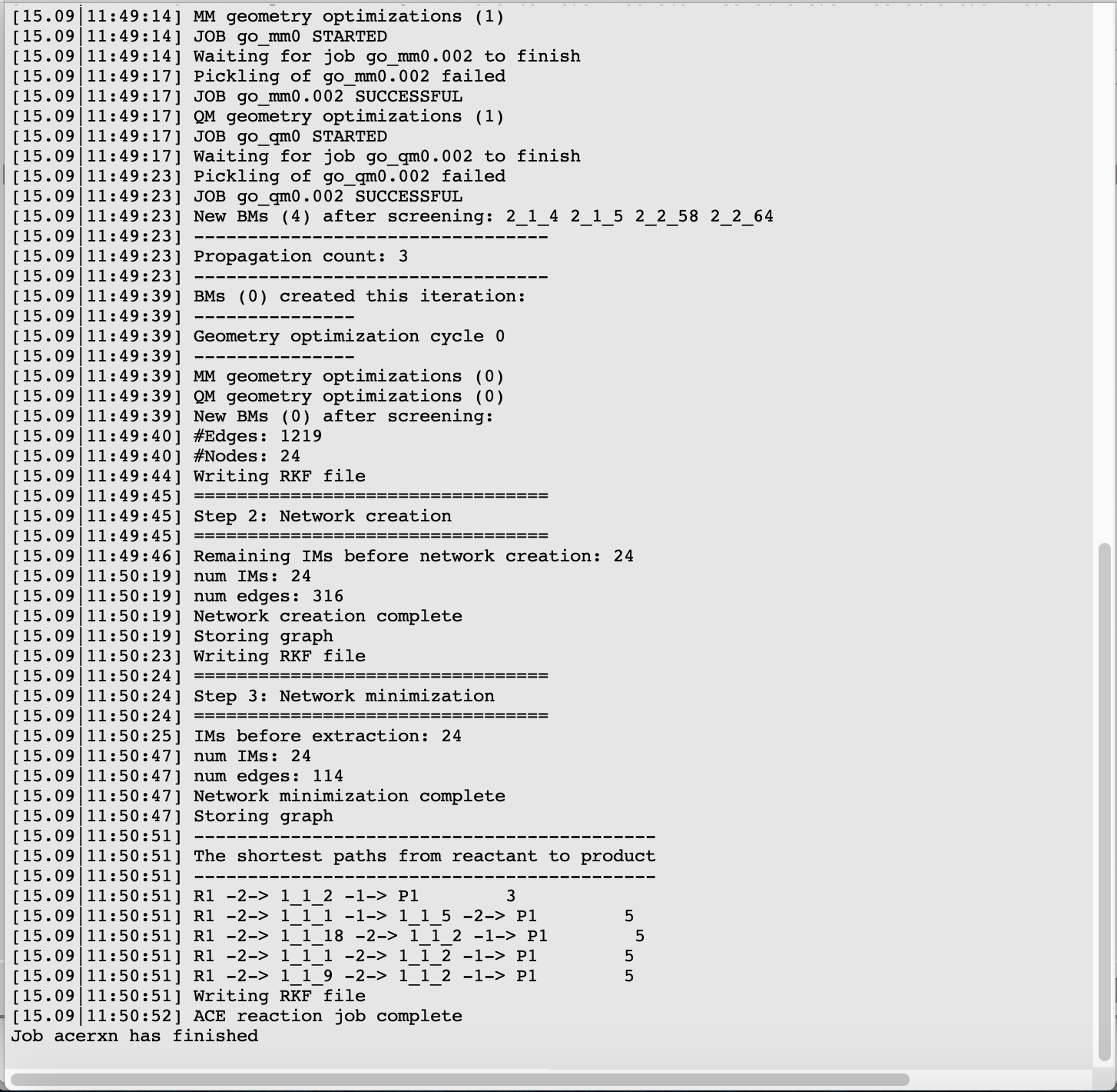
For each of the five paths the names of the intermediates are listed, separated by arrows. At the end of each line, the total number of bonds broken and formed is depicted, which will be referred to as the chemical distance. Inside each arrow, the chemical distance of the elementary reaction is shown.
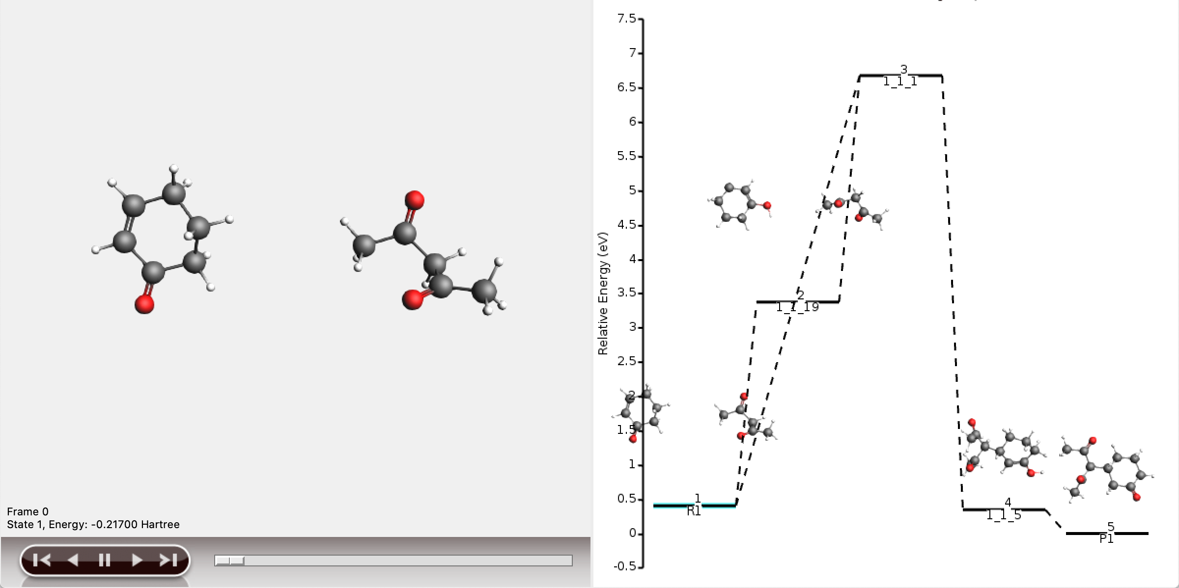
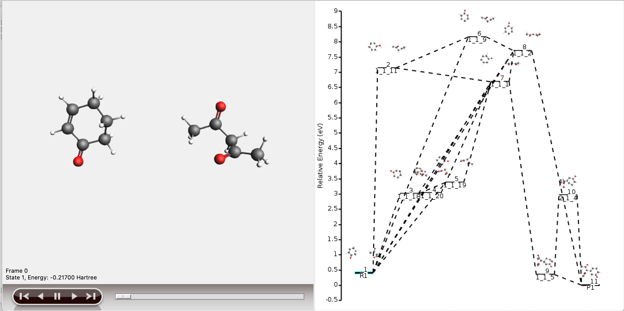
The shortest path has an overall chemical distance of 3, and involves intermediate 1_1_2. A quick look at AMSmovie shows that while this path is the shortest, it is not the lowest energy path.
The lowest energy path connects the reactant (R1) and product (P1) via the two intermediates 1_1_1 and 1_1_5, and has an overall chemical distance of 5.
The reaction diagram in AMSmovie shows that intermediate 1_1_1 corresponds to state 5, and intermediate 1_1_5 corresponds to state 6. In the left panel of the AMSmovie window we can scroll to state 5 and state 6 using the scroll bar at the bottom.
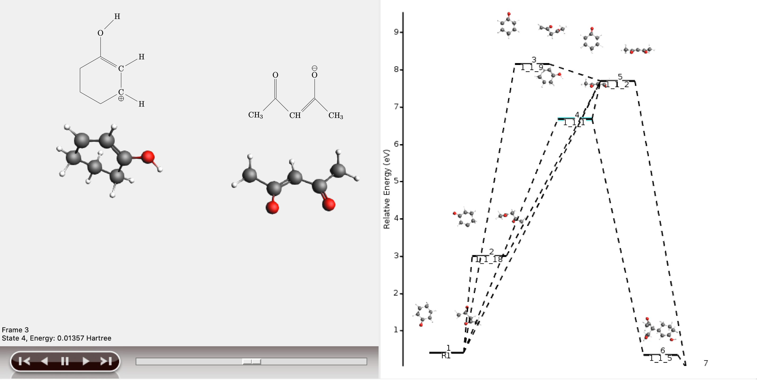
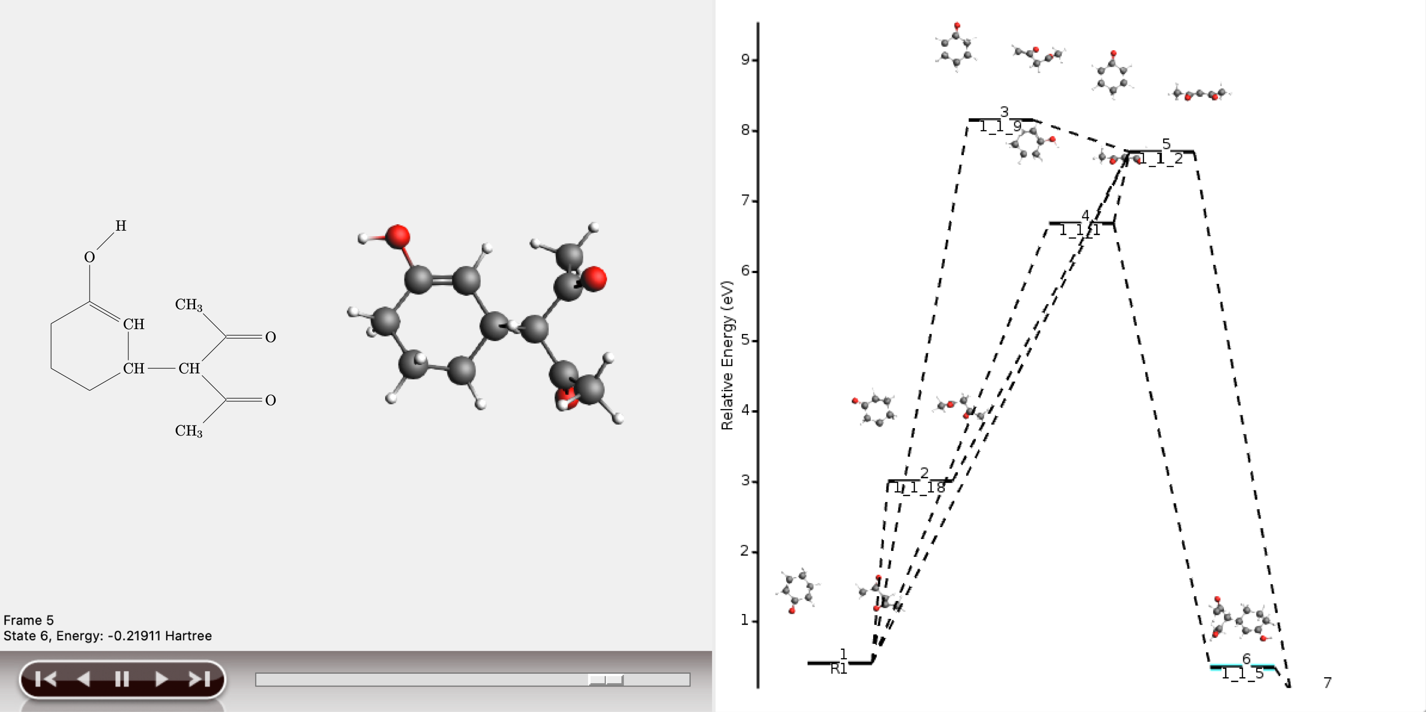
Comparison to our expected reaction mechanism shows that these two intermediates indeed correspond to our expected intermediates, and we can conclude that ACE reaction was able to predict the expected reaction mechanism.
Analyze network
The number of shortest paths printed to logfile and exported to AMSmovie is passed to the job a priori in the settings. Since it is very difficult to visually interpret a network that is too large, the user may want to extract additional paths from the full network a posteriori. This section describes how to do this.
The resulting network as depicted by AMSmovie contains ten paths, and therefore looks complex.
All ten paths are also present in the logfile.
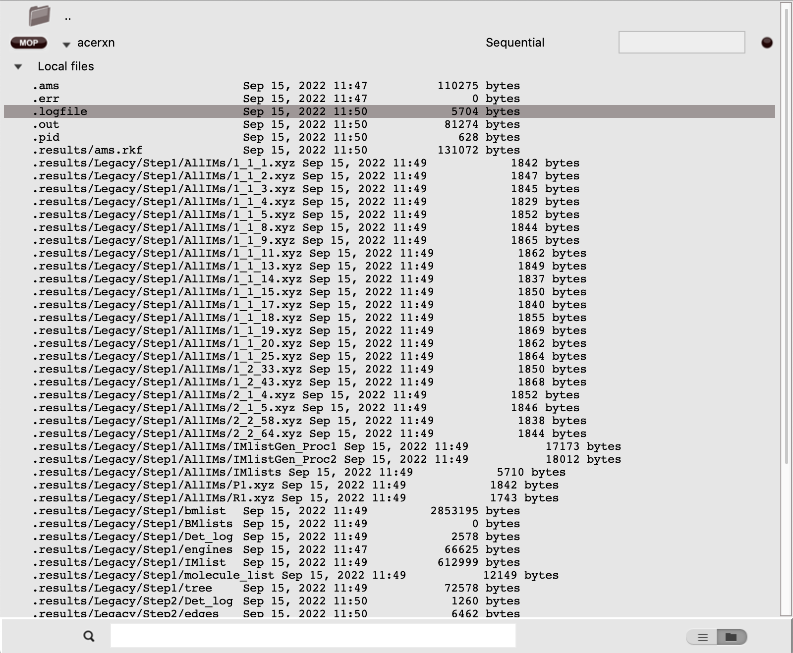
The individual paths have now been stored in the results folder, and can be opened in AMSmovie.
A single path opens in AMSmovie. Compared to path 0, reactions along path 6 are less likely to occur, as it involves an unnecessary intermediate, and can in this case be discarded as an option. More detailed analysis, such as transition state searches, can now focus on the chemically intuitive pathways.