Molecular Dynamics with Python¶

Build a periodic methane box from Python, preoptimize it, and run short NVE, NVT, and NPT molecular-dynamics simulations with the UFF force field. The example shows how to initialize velocities, restart between ensembles, and inspect energies, temperature, pressure, and density directly from the trajectory data.

Downloads: Notebook | Script ?

../_images/molecular_dynamics_intro_76_0_df834b59.png

Initial imports¶

from scm.plams import *
import os
import numpy as np
import matplotlib.pyplot as plt

Create a box of methane¶

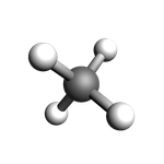
First, create a gasphase methane molecule:

single_molecule = from_smiles(
    "C", forcefield="uff"
)  # or use Molecule('your-own-file.xyz')
view(single_molecule, height=150, width=150)

[10.04|11:23:38] Starting Xvfb...
[10.04|11:23:38] Xvfb started

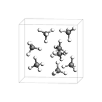
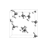
You can easily create a box with a liquid or gas of a given density. For more advanced options, see the Packmol example.

box = packmol(
    single_molecule,
    n_molecules=8,
    region_names="methane",
    density=0.4,  # g/cm^3
)
print("Lattice vectors of the box:\n{}".format(box.lattice))
view(box, height=200, width=200, direction="tilt_z")

Lattice vectors of the box:
[[8.106820570931148, 0.0, 0.0], [0.0, 8.106820570931148, 0.0], [0.0, 0.0, 8.106820570931148]]

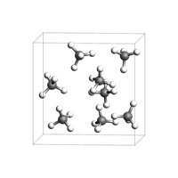
Before running an MD simulation, it is usually a good idea to do a quick geometry optimization (preoptimization).

box = preoptimize(box, model="UFF", maxiterations=50)
view(box, height=200, width=200, direction="tilt_z")

Run an NVE simulation with UFF¶

In an NVE simulation, the total energy (kinetic + potential) is constant.

The initial velocities can either be

read from a file (a previous simulation), or
be generated to follow the Maxwell-Boltzmann distribution at a certain temperature.

Here, we will initialize the velocities corresponding to a temperature of 300 K.

s = Settings()
s.input.ForceField.Type = "UFF"
s.runscript.nproc = 1  # run in serial

nve_job = AMSNVEJob(
    molecule=box,
    settings=s,
    name="NVE-sim-1",
    temperature=300,  # initial velocities from Maxwell-Boltzmann distribution, 300 K
    nsteps=1000,
    samplingfreq=50,
    timestep=1.0,  # femtoseconds
)

When calling nve_job.run(), you can set watch=True to interactively see the progress of the MD simulation.

nve_job.run(watch=True);

[10.04|11:23:41] JOB NVE-sim-1 STARTED
[10.04|11:23:41] JOB NVE-sim-1 RUNNING
[10.04|11:23:41] NVE-sim-1: AMS 2026.102  RunTime: Apr10-2026 11:23:41  ShM Nodes: 1  Procs: 1
[10.04|11:23:41] NVE-sim-1: Starting MD calculation:
[10.04|11:23:41] NVE-sim-1: --------------------
... output trimmed ....
[10.04|11:23:42] JOB NVE-sim-1 FINISHED
[10.04|11:23:43] NVE-sim-1:          1000    1000.00     215.      -0.01305         280.709         532.8
[10.04|11:23:43] NVE-sim-1: MD calculation finished.
[10.04|11:23:43] NVE-sim-1: NORMAL TERMINATION
[10.04|11:23:43] JOB NVE-sim-1 SUCCESSFUL

The main output file from an MD simulation is called ams.rkf. It contains the trajectory and other properties (energies, velocities, …). You can open the file

in the AMSmovie graphical user interface to play (visualize) the trajectory.
in the KFbrowser module (expert mode) to find out where on the file various properties are stored.

Call the job.results.rkfpath() method to find out where the file is:

print(nve_job.results.rkfpath())

/Users/ormrodmorley/Documents/code/ams/amshome_fix2026/userdoc/PythonExamples/molecular-dynamics-intro/plams_workdir.002/NVE-sim-1/ams.rkf

Use job.results.readrkf() to directly read from the ams.rkf file:

n_frames = nve_job.results.readrkf("MDHistory", "nEntries")
print("There are {} frames in the trajectory".format(n_frames))

There are 21 frames in the trajectory

Let’s plot the potential, kinetic, and total energies:

def plot_energies(
    job,
    title=None,
    kinetic_energy=True,
    potential_energy=True,
    total_energy=True,
    conserved_energy=False,
):
    time = job.results.get_history_property("Time", "MDHistory")
    fig, ax = plt.subplots(figsize=(5, 3))
    if kinetic_energy:
        kin_e = job.results.get_history_property("KineticEnergy", "MDHistory")
        ax.plot(time, kin_e, label="Kinetic Energy")
    if potential_energy:
        pot_e = job.results.get_history_property("PotentialEnergy", "MDHistory")
        ax.plot(time, pot_e, label="Potential Energy")
    if total_energy:
        tot_e = job.results.get_history_property("TotalEnergy", "MDHistory")
        ax.plot(time, tot_e, label="Total Energy")
    if conserved_energy:
        conserved_e = job.results.get_history_property("ConservedEnergy", "MDHistory")
        ax.plot(time, conserved_e, label="Conserved Energy")
    ax.legend()
    ax.set_xlabel("Time (fs)")
    ax.set_ylabel("Energy (Ha)")
    ax.set_title(title or job.name + " Energies")
    return ax

ax = plot_energies(nve_job)
ax;

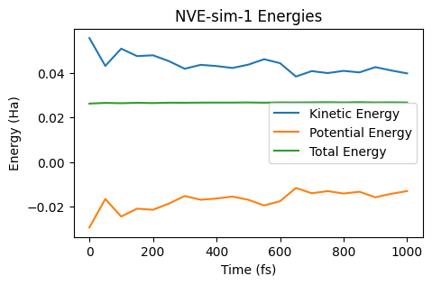
During the NVE simulation, kinetic energy is converted into potential energy and vice versa, but the total energy remains constant.

Let’s also show an image of the final frame. The atoms of some molecules are split across the periodic boundary.

view(nve_job.results.get_main_molecule(), height=200, width=200, direction="tilt_z")

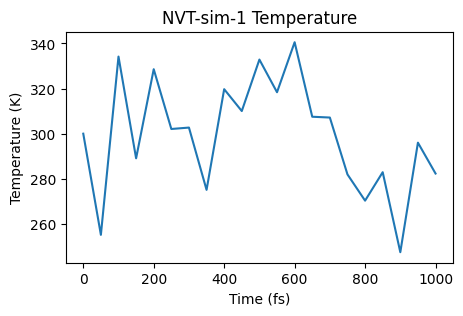
NVT simulation¶

In an NVT simulation, a thermostat keeps the temperature (kinetic energy) in check. The time constant tau (in femtoseconds) indicates how “strong” the thermostat is. For now, let’s set a Berendsen thermostat with a time constant of 100 fs.

nvt_job = AMSNVTJob(
    molecule=box,
    settings=s,
    name="NVT-sim-1",
    nsteps=1000,
    samplingfreq=50,
    timestep=1.0,  # femtoseconds
    temperature=300,
    thermostat="Berendsen",
    tau=100,  # femtoseconds
)
nvt_job.run();

[10.04|11:23:44] JOB NVT-sim-1 STARTED
[10.04|11:23:44] JOB NVT-sim-1 RUNNING
[10.04|11:23:45] JOB NVT-sim-1 FINISHED
[10.04|11:23:45] JOB NVT-sim-1 SUCCESSFUL

def plot_temperature(job, title=None):
    time = job.results.get_history_property("Time", "MDHistory")
    temperature = job.results.get_history_property("Temperature", "MDHistory")
    fig, ax = plt.subplots(figsize=(5, 3))
    ax.plot(time, temperature)
    ax.set_xlabel("Time (fs)")
    ax.set_ylabel("Temperature (K)")
    ax.set_title(title or job.name + " Temperature")
    return ax

ax = plot_temperature(nvt_job)
ax;

ax = plot_energies(nvt_job)
ax;

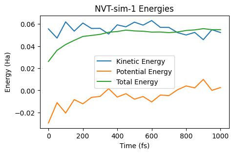
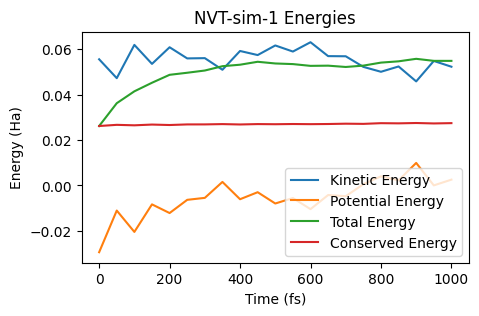
In an NVT simulation, the total energy is not conserved. Instead, the quantity known as “Conserved Energy” is conserved:

ax = plot_energies(nvt_job, conserved_energy=True)
ax;

NPT simulation¶

In an NPT simulation, a barostat is used to keep the pressure constant (fluctuating around a given value). The instantaneous pressure can fluctuate quite wildly, even with a small time constant for the barostat.

Let’s run an NPT simulation with the same thermostat as before and with a barostat set at 1 bar.

Note: It is usually good to pre-equilibrate a simulation in NVT before switching on the barostat. Below we demonstrate the restart_from function, which will restart from nvt_job (final frame and velocities). You can also use restart_from together with AMSNVEJob or AMSNVTJob.

npt_job = AMSNPTJob.restart_from(
    nvt_job,
    name="npt",
    barostat="Berendsen",
    pressure=1e5,  # Pa
    barostat_tau=1000,  # fs
    equal="XYZ",  # scale all lattice vectors equally
)

npt_job.run();

[10.04|11:23:45] JOB npt STARTED
[10.04|11:23:45] JOB npt RUNNING
[10.04|11:23:46] JOB npt FINISHED
[10.04|11:23:46] JOB npt SUCCESSFUL

from scm.plams.tools.postprocess_results import moving_average


def plot_pressure(job, title=None, window: int = None):
    time = job.results.get_history_property("Time", "MDHistory")
    pressure = job.results.get_history_property("Pressure", "MDHistory")
    pressure = Units.convert(pressure, "au", "bar")  # convert from atomic units to bar
    time, pressure = moving_average(time, pressure, window)
    fig, ax = plt.subplots(figsize=(5, 3))
    ax.plot(time, pressure)
    ax.set_xlabel("Time (fs)")
    ax.set_ylabel("Pressure (bar)")
    ax.set_title(title or job.name + " Pressure")
    return ax

ax = plot_pressure(npt_job)
ax;

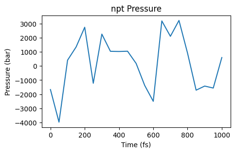
Those are quite some fluctuations! Especially for the pressure it can be useful to plot a moving average. Here the window parameter gives the number of frames in the trajectory to average over.

ax = plot_pressure(npt_job, window=10, title="npt Pressure moving average")
ax;

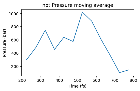
From this moving average it is easier to see that the pressure is too high compared to the target pressure of 1 bar, so the simulation is not yet in equilibrium.

Let’s also plot the density as a function of time:

def plot_density(job, title=None, window: int = None):
    time = job.results.get_history_property("Time", "MDHistory")
    density = job.results.get_history_property("Density", "MDHistory")
    density = (
        np.array(density)
        * Units.convert(1.0, "au", "kg")
        / Units.convert(1.0, "bohr", "m") ** 3
    )
    time, density = moving_average(time, density, window)
    fig, ax = plt.subplots(figsize=(5, 3))
    ax.plot(time, density)
    ax.set_xlabel("Time (fs)")
    ax.set_ylabel("Density (kg/m^3)")
    ax.set_title(title or job.name + " Density")
    return ax

ax = plot_density(npt_job)
ax;

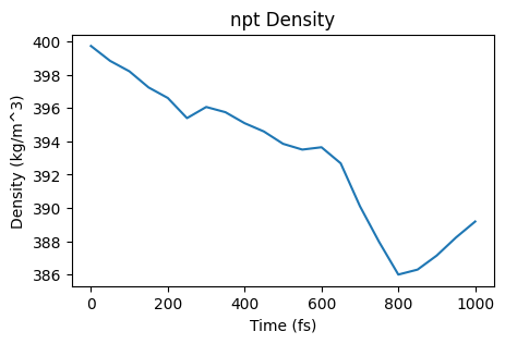
Since the pressure was too high, the barostat increases the size of the simulation box (which decreases the density). Note that the initial density was 400 kg/m^3 which matches the density given to the packmol function at the top (0.4 g/cm^3)!

Equilibration and Mean squared displacement (diffusion coefficient)¶

The mean squared displacement is in practice often calculated from NVT simulations. This is illustrated here. However, best practice is to instead

average over several NVE simulations that have been initialized with velocities from NVT simulations, and to
extrapolate the diffusion coefficient to infinite box size

Those points will be covered later. Here, we just illustrate the simplest possible way (that is also the most common in practice).

The mean squared displacement is only meaningful for fully equilibrated simulations. Let’s first run a reasonably long equilibration simulation, and then a production simulation. These simulations may take a few minutes to complete.

nvt_eq_job = AMSNVTJob(
    molecule=box,
    settings=s,
    name="NVT-equilibration-1",
    temperature=300,
    thermostat="Berendsen",
    tau=200,
    timestep=1.0,
    nsteps=40000,
    samplingfreq=500,
)
nvt_eq_job.run()
ax = plot_energies(nvt_eq_job)
ax;

[10.04|11:23:47] JOB NVT-equilibration-1 STARTED
[10.04|11:23:47] JOB NVT-equilibration-1 RUNNING
[10.04|11:24:26] JOB NVT-equilibration-1 FINISHED
[10.04|11:24:26] JOB NVT-equilibration-1 SUCCESSFUL

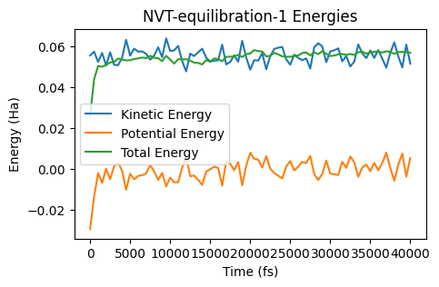
The energies seem equilibrated, so let’s run a production simulation and switch to the NHC (Nose-Hoover) thermostat

nvt_prod_job = AMSNVTJob.restart_from(
    nvt_eq_job,
    name="NVT-production-1",
    nsteps=50000,
    thermostat="NHC",
    samplingfreq=100,
)

nvt_prod_job.run();

[10.04|11:24:26] JOB NVT-production-1 STARTED
[10.04|11:24:26] JOB NVT-production-1 RUNNING
[10.04|11:25:16] JOB NVT-production-1 FINISHED
[10.04|11:25:16] JOB NVT-production-1 SUCCESSFUL

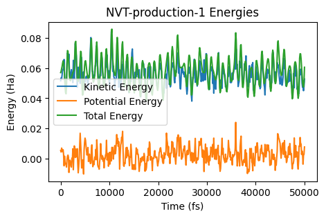
ax = plot_energies(nvt_prod_job)
ax;

ax = plot_temperature(nvt_prod_job)
ax;

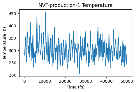
The simulation seems to be sampling an equilibrium distribution, so it’s safe to calculate the mean squared displacement. Let’s use the AMSMSDJob for this. We’ll also specify to only calculate the MSD for the carbon atoms of the methane molecules.

atom_indices = [
    i
    for i, at in enumerate(nvt_prod_job.results.get_main_molecule(), 1)
    if at.symbol == "C"
]
print("Calculating MSD for carbon atoms with indices {}".format(atom_indices))
msd_job = AMSMSDJob(
    nvt_prod_job,
    name="msd-" + nvt_prod_job.name,
    atom_indices=atom_indices,  # indices start with 1 for the first atom
    max_correlation_time_fs=8000,  # max correlation time must be set before running the job
    start_time_fit_fs=3000,  # start_time_fit can also be changed later in the postanalysis
)
msd_job.run();

Calculating MSD for carbon atoms with indices [1, 6, 11, 16, 21, 26, 31, 36]
[10.04|11:25:16] JOB msd-NVT-production-1 STARTED
[10.04|11:25:16] JOB msd-NVT-production-1 RUNNING
[10.04|11:25:16] JOB msd-NVT-production-1 FINISHED
[10.04|11:25:17] JOB msd-NVT-production-1 SUCCESSFUL

def plot_msd(job, start_time_fit_fs=None):
    """job: an AMSMSDJob"""
    time, msd = job.results.get_msd()
    fit_result, fit_x, fit_y = job.results.get_linear_fit(
        start_time_fit_fs=start_time_fit_fs
    )
    # the diffusion coefficient can also be calculated as fit_result.slope/6 (ang^2/fs)
    diffusion_coefficient = job.results.get_diffusion_coefficient(
        start_time_fit_fs=start_time_fit_fs
    )  # m^2/s
    fig, ax = plt.subplots(figsize=(5, 3))
    ax.plot(time, msd, label="MSD")
    ax.plot(
        fit_x, fit_y, label="Linear fit slope={:.5f} ang^2/fs".format(fit_result.slope)
    )
    ax.legend()
    ax.set_xlabel("Correlation time (fs)")
    ax.set_ylabel("Mean square displacement (ang^2)")
    ax.set_title(
        "MSD: Diffusion coefficient = {:.2e} m^2/s".format(diffusion_coefficient)
    )
    return ax

ax = plot_msd(msd_job)
ax;

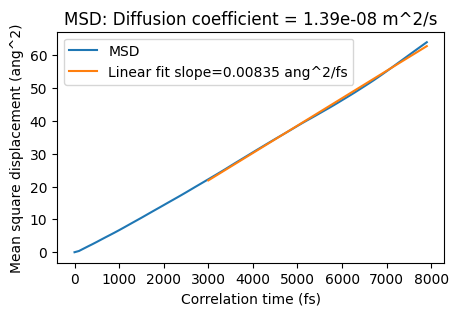
In the above graph, the MSD is a straight line. That is a good sign. If the line isn’t straight at large correlation times, you would need to run a longer simulation. The diffusion coefficient = slope/6.

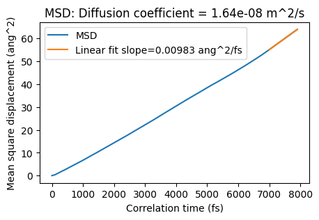
The plot ends at 8000 fs (max_correlation_time_fs), and the linear fit is started from 3000 fs (start_time_fit_fs). You can also change the start of the linear fit in the postprocessing:

plot_msd(msd_job, start_time_fit_fs=7000);

Radial distribution function¶

Similarly to the MSD, a radial distribution function (RDF) should only be calculated for an equilibrated simulation.

Let’s calculate and plot the C-H RDF. Note that the RDF should only be calculated for distances up to half the shortest lattice vector length (for orthorhombic cells).

mol = nvt_prod_job.results.get_main_molecule()
atom_indices = [i for i, at in enumerate(mol, 1) if at.symbol == "C"]
atom_indices_to = [i for i, at in enumerate(mol, 1) if at.symbol == "H"]

# rmax = half the shortest box length for orthorhombic cells
rmax = min([mol.lattice[0][0], mol.lattice[1][1], mol.lattice[2][2]]) / 2

rdf_job = AMSRDFJob(
    nvt_prod_job,
    name="rdf-C-H-" + nvt_prod_job.name,
    atom_indices=atom_indices,  # from C
    atom_indices_to=atom_indices_to,  # to H
    rmin=0.5,
    rmax=rmax,
    rstep=0.1,
)
rdf_job.run();

[10.04|11:25:17] JOB rdf-C-H-NVT-production-1 STARTED
[10.04|11:25:17] JOB rdf-C-H-NVT-production-1 RUNNING
[10.04|11:25:17] JOB rdf-C-H-NVT-production-1 FINISHED
[10.04|11:25:17] JOB rdf-C-H-NVT-production-1 SUCCESSFUL

def plot_rdf(job, title=""):
    fig, ax = plt.subplots(figsize=(5, 3))
    r, rdf = job.results.get_rdf()
    ax.plot(r, rdf)
    ax.set_xlabel("r (angstrom)")
    ax.set_ylabel("g(r)")
    ax.set_title(title or job.name + " RDF")
    return ax

ax = plot_rdf(rdf_job)
ax;

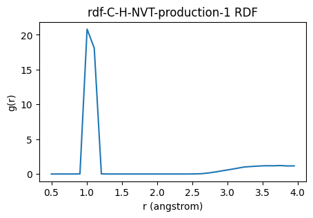
The covalent C-H bonds give rise to the peak slightly above 1.0 angstrom. The RDF then slowly approaches a value of 1, which is the expected value for an ideal gas.

Relation to AMSJob and AMSAnalysisJob¶

The AMSNVEJob, AMSNVTJob, and AMSNPTJob classes are just like normal AMSJob. The arguments populate the job’s settings.

Similarly, AMSMSDJob, AMSRDFJob, and AMSVACFJob are normal AMSAnalysisJob.

Let’s print the AMS input for the nvt_prod_job. Note that the initial velocities (and the structure) come from the equilibration job.

print(nvt_prod_job.get_input())

MolecularDynamics
  BinLog
    DipoleMoment False
    PressureTensor False
    Time False
... output trimmed ....
Engine ForceField
  Type UFF
EndEngine

And similarly the input to the AMS MD postanalysis program for the msd_job:

print(msd_job.get_input())

MeanSquareDisplacement
  Atoms
    Atom 1
    Atom 6
    Atom 11
... output trimmed ....
    KFFilename /Users/ormrodmorley/Documents/code/ams/amshome_fix2026/userdoc/PythonExamples/molecular-dynamics-intro/plams_workdir.002/NVT-production-1/ams.rkf
  end
end

Velocity autocorrelation function, power spectrum, AMSNVESpawner¶

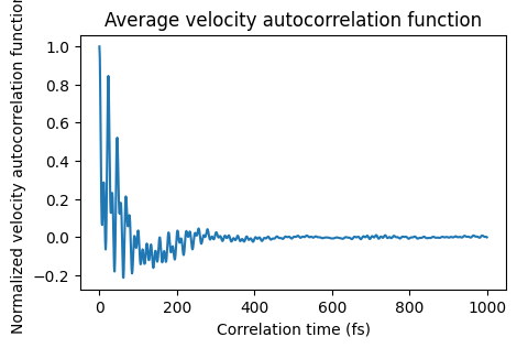
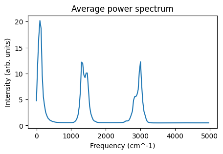
The Fourier transform of the velocity autocorrelation function gives the power spectrum, containing characteristic frequencies of all the vibrations, rotations, and translations of the molecules.

To calculate the velocity autocorrelation function, you need to

run several short NVE simulations with equilibrated initial velocities
write the velocities to disk every step
calculate the autocorrelation function

For the first two steps, we’ll use the AMSNVESpawnerJob class, initializing NVE simulations from evenly spaced frames in the nvt_prod_job job. For the last step, we’ll use the AMSVACFJob.

nvespawner_job = AMSNVESpawnerJob(
    nvt_prod_job,
    name="nvespawner-" + nvt_prod_job.name,
    n_nve=3,  # the number of NVE simulations to run
    samplingfreq=1,  # write to disk every frame for velocity autocorrelation
    writevelocities=True,
    timestep=1.0,  # ideally use smaller timestep
    nsteps=3000,  # 3000 steps (here = 3000 fs) is very short, for demonstration purposes only
)
nvespawner_job.run();

[10.04|11:25:17] JOB nvespawner-NVT-production-1 STARTED
[10.04|11:25:17] JOB nvespawner-NVT-production-1 RUNNING
[10.04|11:25:17] JOB nvespawner-NVT-production-1/nve1 STARTED
[10.04|11:25:17] JOB nvespawner-NVT-production-1/nve1 RUNNING
[10.04|11:25:23] JOB nvespawner-NVT-production-1/nve1 FINISHED
... output trimmed ....
[10.04|11:25:29] JOB nvespawner-NVT-production-1/nve3 RUNNING
[10.04|11:25:36] JOB nvespawner-NVT-production-1/nve3 FINISHED
[10.04|11:25:36] JOB nvespawner-NVT-production-1/nve3 SUCCESSFUL
[10.04|11:25:36] JOB nvespawner-NVT-production-1 FINISHED
[10.04|11:25:38] JOB nvespawner-NVT-production-1 SUCCESSFUL

Let’s then create the AMSVACFJobs. The previous NVE jobs are accessed by nvespawner_job.children.values():

vacf_jobs = []
for job in nvespawner_job.children.values():
    vacf_job = AMSVACFJob(
        job,
        name="vacf-" + job.name + "-" + nvespawner_job.name,
        max_correlation_time_fs=1000,  # 1000 fs is very short, for demo purposes only
    )
    vacf_jobs.append(vacf_job)
    vacf_jobs[-1].run()

[10.04|11:25:38] JOB vacf-nve1-nvespawner-NVT-production-1 STARTED
[10.04|11:25:38] JOB vacf-nve1-nvespawner-NVT-production-1 RUNNING
[10.04|11:25:38] JOB vacf-nve1-nvespawner-NVT-production-1 FINISHED
[10.04|11:25:39] JOB vacf-nve1-nvespawner-NVT-production-1 SUCCESSFUL
[10.04|11:25:39] JOB vacf-nve2-nvespawner-NVT-production-1 STARTED
... output trimmed ....
[10.04|11:25:40] JOB vacf-nve2-nvespawner-NVT-production-1 SUCCESSFUL
[10.04|11:25:40] JOB vacf-nve3-nvespawner-NVT-production-1 STARTED
[10.04|11:25:40] JOB vacf-nve3-nvespawner-NVT-production-1 RUNNING
[10.04|11:25:41] JOB vacf-nve3-nvespawner-NVT-production-1 FINISHED
[10.04|11:25:41] JOB vacf-nve3-nvespawner-NVT-production-1 SUCCESSFUL

Let’s get and plot the average velocity autocorrelation function and power spectrum

def plot_vacf(vacf_jobs):
    """vacf_jobs is a list of AMSVACFJob, plot the average velocity autocorrelation function"""
    x, y = zip(*[job.results.get_vacf() for job in vacf_jobs])
    x = np.mean(x, axis=0)
    y = np.mean(y, axis=0)
    fig, ax = plt.subplots(figsize=(5, 3))
    ax.plot(x, y)
    ax.set_xlabel("Correlation time (fs)")
    ax.set_ylabel("Normalized velocity autocorrelation function")
    ax.set_title("Average velocity autocorrelation function")
    return ax


def plot_power_spectrum(vacf_jobs, ax=None):
    x, y = zip(*[job.results.get_power_spectrum() for job in vacf_jobs])
    x = np.mean(x, axis=0)
    y = np.mean(y, axis=0)
    if ax is None:
        fig, ax = plt.subplots(figsize=(5, 3))
    ax.plot(x, y)
    ax.set_xlabel("Frequency (cm^-1)")
    ax.set_ylabel("Intensity (arb. units)")
    ax.set_title("Average power spectrum")
    return ax

ax = plot_vacf(vacf_jobs)
ax;

ax = plot_power_spectrum(vacf_jobs)
ax;

Let’s compare the power spectrum to the calculated frequencies from a gasphase geometry optimization + frequencies calculation (harmonic approximation). First, let’s define and run the job. Remember: s is the UFF settings from before, and single_molecule is the single methane molecule defined before.

sfreq = Settings()
sfreq.input.ams.Task = "GeometryOptimization"
sfreq.input.ams.Properties.NormalModes = "Yes"
sfreq += s  # UFF engine settings used before
freq_job = AMSJob(
    settings=sfreq, name="methane-optfreq", molecule=single_molecule
)  # single_molecule defined at the beginning
freq_job.run()
print("Normal modes stored in {}".format(freq_job.results.rkfpath(file="engine")))

[10.04|11:25:41] JOB methane-optfreq STARTED
[10.04|11:25:41] JOB methane-optfreq RUNNING
[10.04|11:25:42] JOB methane-optfreq FINISHED
[10.04|11:25:42] JOB methane-optfreq SUCCESSFUL
Normal modes stored in /Users/ormrodmorley/Documents/code/ams/amshome_fix2026/userdoc/PythonExamples/molecular-dynamics-intro/plams_workdir.002/methane-optfreq/forcefield.rkf

You can open the forcefield.rkf file in AMSspectra to visualize the vibrational normal modes. You can also access the frequencies in Python:

freqs = freq_job.results.get_frequencies()
print("There are {} frequencies for gasphase methane".format(len(freqs)))
for f in freqs:
    print("{:.1f} cm^-1".format(f))

There are 9 frequencies for gasphase methane
1 cm^-1
1 cm^-1
1 cm^-1
4 cm^-1
4 cm^-1
4 cm^-1
0 cm^-1
0 cm^-1
0 cm^-1

Let’s make something similar to a power spectrum by placing a Gaussian at each normal mode frequency and compare to the power spectrum from the molecular dynamics.

First, define the gaussian and sumgaussians function to sum up Gaussian functions along an axis:

def gaussian(x, a, b, c):
    return a * np.exp(-((x - b) ** 2) / (2 * c**2))


def sumgaussians(x, a, b, c):
    # calculate the sum of gaussians centered at b for the different x values
    # use numpy array broadcasting by placing x in a row and b in a column
    x = np.reshape(x, (1, -1))  # row
    b = np.reshape(b, (-1, 1))  # column
    return np.sum(gaussian(x, a, b, c), axis=0)

Then, define the x-axis x, and calculate the spectrum from the frequencies by placing gaussians centered at freqs with height controlled by a and width controlled by c:

x = np.arange(5000)  # x axis
y = sumgaussians(x, a=2, b=freqs, c=30)  # intensities, use suitable numbers for a and c

Then compare to the power spectrum from MD:

ax = plot_power_spectrum(vacf_jobs)
ax.plot(x, y)
ax.legend(["power spectrum from MD", "gasphase optimization"]);

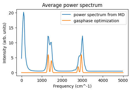
The most striking difference is the intensity below 500 cm^-1 for the MD simulation. This arises from translational and rotational motion. There are also differences in the other peaks, arising from

intermolecular interactions, and
anharmonicity, and
sampling during the MD simulation

Note that the intensity is arbitrarily scaled for both the MD simulation and the gasphase optimization. The above do not correspond to IR or Raman spectra. They are power spectra.

Further molecular-dynamics examples¶

The ReaxFF density-equilibration workflow and the Lennard-Jones diffusion extrapolation workflows are now available as separate self-contained Python examples. See the related-example links on this page for the split-off notebooks.

Python Script¶

#!/usr/bin/env python
# coding: utf-8

# ## Initial imports

from scm.plams import *
import os
import numpy as np
import matplotlib.pyplot as plt


# ## Create a box of methane
#
#
# First, create a gasphase methane molecule:

single_molecule = from_smiles("C", forcefield="uff")  # or use Molecule('your-own-file.xyz')
view(single_molecule, height=150, width=150, picture_path="picture1.png")


# You can easily create a box with a liquid or gas of a given density. For more advanced options, see the Packmol example.

box = packmol(
    single_molecule,
    n_molecules=8,
    region_names="methane",
    density=0.4,  # g/cm^3
)
print("Lattice vectors of the box:\n{}".format(box.lattice))
view(box, height=200, width=200, direction="tilt_z", picture_path="picture2.png")


# Before running an MD simulation, it is usually a good idea to do a quick geometry optimization (preoptimization).

box = preoptimize(box, model="UFF", maxiterations=50)
view(box, height=200, width=200, direction="tilt_z", picture_path="picture3.png")


# ### Run an NVE simulation with UFF
#
# In an NVE simulation, the total energy (kinetic + potential) is constant.
#
# The initial velocities can either be
#
# * read from a file (a previous simulation), or
#
# * be generated to follow the Maxwell-Boltzmann distribution at a certain temperature.
#
# Here, we will initialize the velocities corresponding to a temperature of 300 K.

s = Settings()
s.input.ForceField.Type = "UFF"
s.runscript.nproc = 1  # run in serial

nve_job = AMSNVEJob(
    molecule=box,
    settings=s,
    name="NVE-sim-1",
    temperature=300,  # initial velocities from Maxwell-Boltzmann distribution, 300 K
    nsteps=1000,
    samplingfreq=50,
    timestep=1.0,  # femtoseconds
)


# When calling ``nve_job.run()``, you can set ``watch=True`` to interactively see the progress of the MD simulation.

nve_job.run(watch=True)
# The main output file from an MD simulation is called **ams.rkf**. It contains the trajectory and other properties (energies, velocities, ...). You can open the file
#
# * in the AMSmovie graphical user interface to play (visualize) the trajectory.
#
# * in the KFbrowser module (expert mode) to find out where on the file various properties are stored.
#
# Call the ``job.results.rkfpath()`` method to find out where the file is:

print(nve_job.results.rkfpath())


# Use ``job.results.readrkf()`` to directly read from the ams.rkf file:

n_frames = nve_job.results.readrkf("MDHistory", "nEntries")
print("There are {} frames in the trajectory".format(n_frames))


# Let's plot the potential, kinetic, and total energies:


def plot_energies(
    job,
    title=None,
    kinetic_energy=True,
    potential_energy=True,
    total_energy=True,
    conserved_energy=False,
):
    time = job.results.get_history_property("Time", "MDHistory")
    fig, ax = plt.subplots(figsize=(5, 3))
    if kinetic_energy:
        kin_e = job.results.get_history_property("KineticEnergy", "MDHistory")
        ax.plot(time, kin_e, label="Kinetic Energy")
    if potential_energy:
        pot_e = job.results.get_history_property("PotentialEnergy", "MDHistory")
        ax.plot(time, pot_e, label="Potential Energy")
    if total_energy:
        tot_e = job.results.get_history_property("TotalEnergy", "MDHistory")
        ax.plot(time, tot_e, label="Total Energy")
    if conserved_energy:
        conserved_e = job.results.get_history_property("ConservedEnergy", "MDHistory")
        ax.plot(time, conserved_e, label="Conserved Energy")
    ax.legend()
    ax.set_xlabel("Time (fs)")
    ax.set_ylabel("Energy (Ha)")
    ax.set_title(title or job.name + " Energies")
    return ax


ax = plot_energies(nve_job)
ax
ax.figure.savefig("picture4.png")


# During the NVE simulation, kinetic energy is converted into potential energy and vice versa, but the total energy remains constant.
#
# Let's also show an image of the final frame. The atoms of some molecules are split across the periodic boundary.

view(nve_job.results.get_main_molecule(), height=200, width=200, direction="tilt_z", picture_path="picture5.png")


# ## NVT simulation
#
# In an NVT simulation, a thermostat keeps the temperature (kinetic energy) in check. The time constant tau (in femtoseconds) indicates how "strong" the thermostat is. For now, let's set a Berendsen thermostat with a time constant of 100 fs.

nvt_job = AMSNVTJob(
    molecule=box,
    settings=s,
    name="NVT-sim-1",
    nsteps=1000,
    samplingfreq=50,
    timestep=1.0,  # femtoseconds
    temperature=300,
    thermostat="Berendsen",
    tau=100,  # femtoseconds
)
nvt_job.run()


def plot_temperature(job, title=None):
    time = job.results.get_history_property("Time", "MDHistory")
    temperature = job.results.get_history_property("Temperature", "MDHistory")
    fig, ax = plt.subplots(figsize=(5, 3))
    ax.plot(time, temperature)
    ax.set_xlabel("Time (fs)")
    ax.set_ylabel("Temperature (K)")
    ax.set_title(title or job.name + " Temperature")
    return ax


ax = plot_temperature(nvt_job)
ax
ax.figure.savefig("picture6.png")


ax = plot_energies(nvt_job)
ax
ax.figure.savefig("picture7.png")


# In an NVT simulation, the total energy is not conserved. Instead, the quantity known as "Conserved Energy" is conserved:

ax = plot_energies(nvt_job, conserved_energy=True)
ax
ax.figure.savefig("picture8.png")


# ## NPT simulation
#
# In an NPT simulation, a barostat is used to keep the pressure constant (fluctuating around a given value). The instantaneous pressure can fluctuate quite wildly, even with a small time constant for the barostat.
#
# Let's run an NPT simulation with the same thermostat as before and with a barostat set at 1 bar.
#
# **Note**: It is usually good to pre-equilibrate a simulation in NVT before switching on the barostat. Below we demonstrate the ``restart_from`` function, which will restart from ``nvt_job`` (final frame and velocities). You can also use ``restart_from`` together with AMSNVEJob or AMSNVTJob.

npt_job = AMSNPTJob.restart_from(
    nvt_job,
    name="npt",
    barostat="Berendsen",
    pressure=1e5,  # Pa
    barostat_tau=1000,  # fs
    equal="XYZ",  # scale all lattice vectors equally
)

npt_job.run()
from scm.plams.tools.postprocess_results import moving_average


def plot_pressure(job, title=None, window: int = None):
    time = job.results.get_history_property("Time", "MDHistory")
    pressure = job.results.get_history_property("Pressure", "MDHistory")
    pressure = Units.convert(pressure, "au", "bar")  # convert from atomic units to bar
    time, pressure = moving_average(time, pressure, window)
    fig, ax = plt.subplots(figsize=(5, 3))
    ax.plot(time, pressure)
    ax.set_xlabel("Time (fs)")
    ax.set_ylabel("Pressure (bar)")
    ax.set_title(title or job.name + " Pressure")
    return ax


ax = plot_pressure(npt_job)
ax
ax.figure.savefig("picture9.png")


# Those are quite some fluctuations! Especially for the pressure it can be useful to **plot a moving average**. Here the ``window`` parameter gives the number of frames in the trajectory to average over.

ax = plot_pressure(npt_job, window=10, title="npt Pressure moving average")
ax
ax.figure.savefig("picture10.png")


# From this moving average it is easier to see that the pressure is too high compared to the target pressure of 1 bar, so the simulation is not yet in equilibrium.
#
# Let's also plot the density as a function of time:


def plot_density(job, title=None, window: int = None):
    time = job.results.get_history_property("Time", "MDHistory")
    density = job.results.get_history_property("Density", "MDHistory")
    density = np.array(density) * Units.convert(1.0, "au", "kg") / Units.convert(1.0, "bohr", "m") ** 3
    time, density = moving_average(time, density, window)
    fig, ax = plt.subplots(figsize=(5, 3))
    ax.plot(time, density)
    ax.set_xlabel("Time (fs)")
    ax.set_ylabel("Density (kg/m^3)")
    ax.set_title(title or job.name + " Density")
    return ax


ax = plot_density(npt_job)
ax
ax.figure.savefig("picture11.png")


# Since the pressure was too high, the barostat increases the size of the simulation box (which decreases the density). Note that the initial density was 400 kg/m^3 which matches the density given to the ``packmol`` function at the top (0.4 g/cm^3)!

# ## Equilibration and Mean squared displacement (diffusion coefficient)
#
# The mean squared displacement is in practice often calculated from NVT simulations. This is illustrated here. However, best practice is to instead
#
# * average over several NVE simulations that have been initialized with velocities from NVT simulations, and to
# * extrapolate the diffusion coefficient to infinite box size
#
# Those points will be covered later. Here, we just illustrate the simplest possible way (that is also the most common in practice).
#
# The mean squared displacement is only meaningful for fully **equilibrated** simulations. Let's first run a reasonably long equilibration simulation, and then a production simulation. These simulations may take a few minutes to complete.

nvt_eq_job = AMSNVTJob(
    molecule=box,
    settings=s,
    name="NVT-equilibration-1",
    temperature=300,
    thermostat="Berendsen",
    tau=200,
    timestep=1.0,
    nsteps=40000,
    samplingfreq=500,
)
nvt_eq_job.run()
ax = plot_energies(nvt_eq_job)
ax
ax.figure.savefig("picture12.png")


# The energies seem equilibrated, so let's run a production simulation and switch to the NHC (Nose-Hoover) thermostat

nvt_prod_job = AMSNVTJob.restart_from(
    nvt_eq_job,
    name="NVT-production-1",
    nsteps=50000,
    thermostat="NHC",
    samplingfreq=100,
)

nvt_prod_job.run()
ax = plot_energies(nvt_prod_job)
ax
ax.figure.savefig("picture13.png")


ax = plot_temperature(nvt_prod_job)
ax
ax.figure.savefig("picture14.png")


# The simulation seems to be sampling an equilibrium distribution, so it's safe to calculate the mean squared displacement. Let's use the ``AMSMSDJob`` for this. We'll also specify to only calculate the MSD for the carbon atoms of the methane molecules.

atom_indices = [i for i, at in enumerate(nvt_prod_job.results.get_main_molecule(), 1) if at.symbol == "C"]
print("Calculating MSD for carbon atoms with indices {}".format(atom_indices))
msd_job = AMSMSDJob(
    nvt_prod_job,
    name="msd-" + nvt_prod_job.name,
    atom_indices=atom_indices,  # indices start with 1 for the first atom
    max_correlation_time_fs=8000,  # max correlation time must be set before running the job
    start_time_fit_fs=3000,  # start_time_fit can also be changed later in the postanalysis
)
msd_job.run()


def plot_msd(job, start_time_fit_fs=None):
    """job: an AMSMSDJob"""
    time, msd = job.results.get_msd()
    fit_result, fit_x, fit_y = job.results.get_linear_fit(start_time_fit_fs=start_time_fit_fs)
    # the diffusion coefficient can also be calculated as fit_result.slope/6 (ang^2/fs)
    diffusion_coefficient = job.results.get_diffusion_coefficient(start_time_fit_fs=start_time_fit_fs)  # m^2/s
    fig, ax = plt.subplots(figsize=(5, 3))
    ax.plot(time, msd, label="MSD")
    ax.plot(fit_x, fit_y, label="Linear fit slope={:.5f} ang^2/fs".format(fit_result.slope))
    ax.legend()
    ax.set_xlabel("Correlation time (fs)")
    ax.set_ylabel("Mean square displacement (ang^2)")
    ax.set_title("MSD: Diffusion coefficient = {:.2e} m^2/s".format(diffusion_coefficient))
    return ax


ax = plot_msd(msd_job)
ax
ax.figure.savefig("picture15.png")


# In the above graph, the MSD is a straight line. That is a good sign. If the line isn't straight at large correlation times, you would need to run a longer simulation. The diffusion coefficient = slope/6.
#
# The plot ends at 8000 fs (``max_correlation_time_fs``), and the linear fit is started from 3000 fs (``start_time_fit_fs``). You can also change the start of the linear fit in the postprocessing:

plot_msd(msd_job, start_time_fit_fs=7000)
# ## Radial distribution function
#
# Similarly to the MSD, a radial distribution function (RDF) should only be calculated for an **equilibrated** simulation.
#
# Let's calculate and plot the C-H RDF. Note that the RDF should only be calculated for distances up to half the shortest lattice vector length (for orthorhombic cells).

mol = nvt_prod_job.results.get_main_molecule()
atom_indices = [i for i, at in enumerate(mol, 1) if at.symbol == "C"]
atom_indices_to = [i for i, at in enumerate(mol, 1) if at.symbol == "H"]

# rmax = half the shortest box length for orthorhombic cells
rmax = min([mol.lattice[0][0], mol.lattice[1][1], mol.lattice[2][2]]) / 2

rdf_job = AMSRDFJob(
    nvt_prod_job,
    name="rdf-C-H-" + nvt_prod_job.name,
    atom_indices=atom_indices,  # from C
    atom_indices_to=atom_indices_to,  # to H
    rmin=0.5,
    rmax=rmax,
    rstep=0.1,
)
rdf_job.run()


def plot_rdf(job, title=""):
    fig, ax = plt.subplots(figsize=(5, 3))
    r, rdf = job.results.get_rdf()
    ax.plot(r, rdf)
    ax.set_xlabel("r (angstrom)")
    ax.set_ylabel("g(r)")
    ax.set_title(title or job.name + " RDF")
    return ax


ax = plot_rdf(rdf_job)
ax
ax.figure.savefig("picture16.png")


# The covalent C-H bonds give rise to the peak slightly above 1.0 angstrom. The RDF then slowly approaches a value of 1, which is the expected value for an ideal gas.

# ## Relation to AMSJob and AMSAnalysisJob
#
# The ``AMSNVEJob``, ``AMSNVTJob``, and ``AMSNPTJob`` classes are just like normal ``AMSJob``. The arguments populate the job's ``settings``.
#
# Similarly, ``AMSMSDJob``, ``AMSRDFJob``, and ``AMSVACFJob`` are normal ``AMSAnalysisJob``.
#
# Let's print the AMS input for the ``nvt_prod_job``. Note that the initial velocities (and the structure) come from the equilibration job.

print(nvt_prod_job.get_input())


# And similarly the input to the AMS MD postanalysis program for the ``msd_job``:

print(msd_job.get_input())


# ## Velocity autocorrelation function, power spectrum, AMSNVESpawner
#
# The Fourier transform of the velocity autocorrelation function gives the power spectrum, containing characteristic frequencies of all the vibrations, rotations, and translations of the molecules.
#
# To calculate the velocity autocorrelation function, you need to
#
# * run several short NVE simulations with equilibrated initial velocities
# * write the velocities to disk every step
# * calculate the autocorrelation function
#
# For the first two steps, we'll use the ``AMSNVESpawnerJob`` class, initializing NVE simulations from evenly spaced frames in the ``nvt_prod_job`` job. For the last step, we'll use the ``AMSVACFJob``.

nvespawner_job = AMSNVESpawnerJob(
    nvt_prod_job,
    name="nvespawner-" + nvt_prod_job.name,
    n_nve=3,  # the number of NVE simulations to run
    samplingfreq=1,  # write to disk every frame for velocity autocorrelation
    writevelocities=True,
    timestep=1.0,  # ideally use smaller timestep
    nsteps=3000,  # 3000 steps (here = 3000 fs) is very short, for demonstration purposes only
)
nvespawner_job.run()
# Let's then create the AMSVACFJobs. The previous NVE jobs are accessed by ``nvespawner_job.children.values()``:

vacf_jobs = []
for job in nvespawner_job.children.values():
    vacf_job = AMSVACFJob(
        job,
        name="vacf-" + job.name + "-" + nvespawner_job.name,
        max_correlation_time_fs=1000,  # 1000 fs is very short, for demo purposes only
    )
    vacf_jobs.append(vacf_job)
    vacf_jobs[-1].run()


# Let's get and plot the average velocity autocorrelation function and power spectrum


def plot_vacf(vacf_jobs):
    """vacf_jobs is a list of AMSVACFJob, plot the average velocity autocorrelation function"""
    x, y = zip(*[job.results.get_vacf() for job in vacf_jobs])
    x = np.mean(x, axis=0)
    y = np.mean(y, axis=0)
    fig, ax = plt.subplots(figsize=(5, 3))
    ax.plot(x, y)
    ax.set_xlabel("Correlation time (fs)")
    ax.set_ylabel("Normalized velocity autocorrelation function")
    ax.set_title("Average velocity autocorrelation function")
    return ax


def plot_power_spectrum(vacf_jobs, ax=None):
    x, y = zip(*[job.results.get_power_spectrum() for job in vacf_jobs])
    x = np.mean(x, axis=0)
    y = np.mean(y, axis=0)
    if ax is None:
        fig, ax = plt.subplots(figsize=(5, 3))
    ax.plot(x, y)
    ax.set_xlabel("Frequency (cm^-1)")
    ax.set_ylabel("Intensity (arb. units)")
    ax.set_title("Average power spectrum")
    return ax


ax = plot_vacf(vacf_jobs)
ax
ax.figure.savefig("picture17.png")


ax = plot_power_spectrum(vacf_jobs)
ax
ax.figure.savefig("picture18.png")


# Let's compare the power spectrum to the calculated frequencies from a gasphase geometry optimization + frequencies calculation (harmonic approximation). First, let's define and run the job. Remember: ``s`` is the UFF settings from before, and ``single_molecule`` is the single methane molecule defined before.

sfreq = Settings()
sfreq.input.ams.Task = "GeometryOptimization"
sfreq.input.ams.Properties.NormalModes = "Yes"
sfreq += s  # UFF engine settings used before
freq_job = AMSJob(
    settings=sfreq, name="methane-optfreq", molecule=single_molecule
)  # single_molecule defined at the beginning
freq_job.run()
print("Normal modes stored in {}".format(freq_job.results.rkfpath(file="engine")))


# You can open the ``forcefield.rkf`` file in AMSspectra to visualize the vibrational normal modes. You can also access the frequencies in Python:

freqs = freq_job.results.get_frequencies()
print("There are {} frequencies for gasphase methane".format(len(freqs)))
for f in freqs:
    print("{:.1f} cm^-1".format(f))


# Let's make something similar to a power spectrum by placing a Gaussian at each normal mode frequency and compare to the power spectrum from the molecular dynamics.
#
# First, define the ``gaussian`` and ``sumgaussians`` function to sum up Gaussian functions along an axis:


def gaussian(x, a, b, c):
    return a * np.exp(-((x - b) ** 2) / (2 * c**2))


def sumgaussians(x, a, b, c):
    # calculate the sum of gaussians centered at b for the different x values
    # use numpy array broadcasting by placing x in a row and b in a column
    x = np.reshape(x, (1, -1))  # row
    b = np.reshape(b, (-1, 1))  # column
    return np.sum(gaussian(x, a, b, c), axis=0)


# Then, define the x-axis ``x``, and calculate the spectrum from the frequencies by placing gaussians centered at ``freqs`` with height controlled by ``a`` and width controlled by ``c``:

x = np.arange(5000)  # x axis
y = sumgaussians(x, a=2, b=freqs, c=30)  # intensities, use suitable numbers for a and c


# Then compare to the power spectrum from MD:

ax = plot_power_spectrum(vacf_jobs)
ax.plot(x, y)
ax.legend(["power spectrum from MD", "gasphase optimization"])
ax.figure.savefig("picture19.png")


# The most striking difference is the intensity below 500 cm^-1 for the MD simulation. This arises from translational and rotational motion. There are also differences in the other peaks, arising from
#
# * intermolecular interactions, and
# * anharmonicity, and
# * sampling during the MD simulation
#
# Note that the intensity is arbitrarily scaled for both the MD simulation and the gasphase optimization. The above do **not** correspond to IR or Raman spectra. They are power spectra.

# ## Further molecular-dynamics examples
#
# The ReaxFF density-equilibration workflow and the Lennard-Jones diffusion extrapolation workflows are now available as separate self-contained Python examples. See the related-example links on this page for the split-off notebooks.
#