Ziff-Gulari-Barshad Model: Phase Transitions and ML-based Surrogate Model
Note
To follow this tutorial, either:
Download
PhaseTransitions-ADP.py(run as$AMSBIN/amspython PhaseTransitions-ADP.py).Download
PhaseTransitions-ADP.ipynb(see also: how to install Jupyterlab)
We studied the effect of changing the composition of the gas phase, namely partial pressures for \(O_2\) and \(CO\), in the \(CO_2\) Turnover frequency (TOF), in some of the pyZacros tutorials for the Ziff-Gulari-Barshad model (see especially Phase Transitions in the ZGB model and Ziff-Gulari-Barshad model: Steady State Conditions). We used an evenly distributed grid on the \(CO\) gas phase molar fraction in those tutorials. From the results, it is possible to see that, typically, the lower the \(CO_2\) production, the more difficult it is to achieve a steady state (except when \(CO_2\) production is zero, likely because the surface got poisoned, which makes the calculation finish quickly). This means that most of the computational time is spent on points that, from a catalytic standpoint, are not as interesting as points with higher \(CO_2\) production. Thus, to reduce the overall computational cost, it would be ideal to generate more points in the more interesting areas automatically. This is the main goal of the Adaptive Design Procedure (ADP).
The ADP was created to generate training data for Machine Learning (ML) algorithms, with a particular emphasis on approximating computationally-intensive first-principles kinetic models in catalysis. The procedure is based on function topology and behavior, with the discrete gradient and relative importance of the independent variables calculated. See more details in the original publication Chem. Eng. J 400, (2020), 125469. The authors demonstrate that the procedure could design a dataset (achieving the same accuracy) using only between 60 and 80% fewer data points as are needed in an evenly distributed grid. Furthermore, the ADP generates a Surrogate Model of the data based on ML techniques, allowing interpolation of points not included in the original data set, which is critical for multiscale simulations of complex chemical reactors.
In this tutorial, we will likewise examine the effects of altering the gas phase’s composition in the \(CO_2\) Turnover frequency (TOF) in the ZGB model, but we will do so while utilizing the ADP to both suggest the values of the \(CO\) molar fractions to evaluate and generate a surrogate model for this solution. In practice, the surrogate model is a PKL file that contains all of the parameters of the ML model, allowing it to be regenerated and used subsequently. The main goal of this tutorial is to obtain this file.
First of all, we must install the package adaptiveDesignProcedure.
If you are using AMS2026, this is included in the amspython base
stack. Otherwise, you can either follow the install procedure described
in the GitHub repository
https://github.com/mbracconi/adaptiveDesignProcedure, or if you are
using an earlier version of AMS, you can install it via amspackages,
by typing the following in a terminal:
$ amspackages install adaptivedesignprocedure
Now, let’s start with the script. Foremost, we import all packages we need:
import multiprocessing
import numpy

import scm.plams
import scm.pyzacros as pz
import scm.pyzacros.models

import adaptiveDesignProcedure as adp
import warnings

warnings.simplefilter("ignore", UserWarning)
The import warning line is just needed to get clean output messages
further down.
The ADP method needs a function that generates the data for the model;
we named it get_rate(). This function accepts a single argument, a
2d-array containing the conditions to be computed with the shape
(number of conditions, number of input variables), and returns a
2d-array containing the calculated values with the shape
(number of conditions, number of output variables). The number of
conditions will be determined on the fly by the ADP. On the contrary, we
must decide on the number of input and output variables. In our example,
we have one input variable, the molar fraction of CO, and
three output variables, the average coverage for \(O*\) and
\(CO*\) and the \(CO_2\) TOF.
This get_rate() function performs a ZacrosParametersScanJob
calculation. To follow the details, please refer to the example Phase
Transitions in the ZGB model. In a nutshell, it configures the
ZacrosJob calculation with the ZGB predefined model. Then it
configures and runs the ZacrosParametersScanJob, using the
ZacrosJob defined before as the reference and setting the \(CO\)
molar fraction equal to the conditions established by the ADP. Finally,
it retrieves the results for each condition by calling the
turnover frequency() and average coverage() functions and
storing them in the output array in the correct order.
def get_rate(conditions):

    print("")
    print("  Requesting:")
    for cond in conditions:
        print("    x_CO = ", cond[0])
    print("")

    # ---------------------------------------
    # Zacros calculation
    # ---------------------------------------
    zgb = pz.models.ZiffGulariBarshad()

    z_sett = pz.Settings()
    z_sett.random_seed = 953129
    z_sett.temperature = 500.0
    z_sett.pressure = 1.0
    z_sett.species_numbers = ("time", 0.1)
    z_sett.max_time = 10.0

    z_job = pz.ZacrosJob(
        settings=z_sett, lattice=zgb.lattice, mechanism=zgb.mechanism, cluster_expansion=zgb.cluster_expansion
    )

    # ---------------------------------------
    # Parameters scan calculation
    # ---------------------------------------
    ps_params = pz.ZacrosParametersScanJob.Parameters()
    ps_params.add("x_CO", "molar_fraction.CO", [cond[0] for cond in conditions])
    ps_params.add("x_O2", "molar_fraction.O2", lambda params: 1.0 - params["x_CO"])

    ps_job = pz.ZacrosParametersScanJob(reference=z_job, parameters=ps_params)

    # ---------------------------------------
    # Running the calculations
    # ---------------------------------------
    results = ps_job.run()

    if not results.job.ok():
        print("Something went wrong!")

    # ---------------------------------------
    # Collecting the results
    # ---------------------------------------
    data = numpy.nan * numpy.empty((len(conditions), 3))
    if results.job.ok():
        results_dict = results.turnover_frequency()
        results_dict = results.average_coverage(last=20, update=results_dict)

        for i in range(len(results_dict)):
            data[i, 0] = results_dict[i]["average_coverage"]["O*"]
            data[i, 1] = results_dict[i]["average_coverage"]["CO*"]
            data[i, 2] = results_dict[i]["turnover_frequency"]["CO2"]

    return data
Now, let’s look at the script’s main part.
As usual, we initialize the pyZacros environment:
scm.pyzacros.init()
PLAMS working folder: /home/user/pyzacros/examples/ZiffGulariBarshad/plams_workdir
We’ll use the plams.JobRunner class, which easily allows us to run
as many parallel instances as we request. In this case, we choose to use
the maximum number of simultaneous processes (maxjobs) equal to the
number of processors in the machine. Additionally, by setting
nproc = 1 we establish that only one processor will be used for
each zacros instance.
maxjobs = multiprocessing.cpu_count()
scm.plams.config.default_jobrunner = scm.plams.JobRunner(parallel=True, maxjobs=maxjobs)
scm.plams.config.job.runscript.nproc = 1
print("Running up to {} jobs in parallel simultaneously".format(maxjobs))
Running up to 8 jobs in parallel simultaneously
Firstly, we must define the input and output variables. As previously
stated, for the input variables, we only have the molar fraction of CO
(x_CO). In terms of ADP, we must provide a name as well as a range
to cover during the execution, ranging from min to max and
beginning with num evenly spaced samples. Regarding the output
variables, we have three: the average coverage for \(O*\) and
\(CO*\), as well as the \(CO_2\) TOF. For them, in ADP, we only
need to provide their names (ac_O, ac_CO, TOF_CO2). Notice
these names are arbitrary, and they do not have any effect on the final
results. However, the number of input and output variables should be in
correspondence with the array sizes used in the get_rate() function.
input_var = ({"name": "x_CO", "min": 0.2, "max": 0.8, "num": 5},)

output_var = ({"name": "ac_O"}, {"name": "ac_CO"}, {"name": "TOF_CO2"})
Then, we create an adaptativeDesignProcedure object by calling its
constructor, which needs the input and output variables, the function to
calculate the rates get_rates. Additionally, for convenience, we set
the output directory as a subdirectory of the pyZacros working directory
and set the random seed (randomState) to get reproducible results.
The last two parameters are optional. It is also possible to provide
several parameters to control the algorithm using the keyword
``algorithmParams’’. But we will get back to that later.
adpML = adp.adaptiveDesignProcedure(
    input_var, output_var, get_rate, outputDir=scm.pyzacros.workdir() + "/adp.results", randomState=10
)
------ Adaptive generation of Training Data for Machine Learning ------

Input parameters:
  * Forest file: /home/user/pyzacros/examples/ZiffGulariBarshad/plams_workdir/adp.results/ml_ExtraTrees.pkl
  * Training file: /home/user/pyzacros/examples/ZiffGulariBarshad/plams_workdir/adp.results/tmp/train.dat
  * Figure path: /home/user/pyzacros/examples/ZiffGulariBarshad/plams_workdir/adp.results/figures
  * Plotting enabled: False
  * Boruta as feature selector: True
  * Use Weak Support Var in Boruta:True

...

        name: ac_CO
    }
    {
        name: TOF_CO2
    }
Now, we begin the calculation by invoking the method
createTrainingDataAndML(), which, as the name implies, generates the
training data as well as the surrogate model (or ML model). The program
runs several cycles, and for each cycle, increases the number of points
and calls the “get rate()” function to evaluate them. When the Relative
Approximation Error and the Out-Of-Bag error are less than
algorithmParams['RADth'] (default=10%) and
algorithmParams['OOBth'] (default=0.05), respectively, the
calculation converges. See the original ADP documentation for more
details.
adpML.createTrainingDataAndML()
------------------ Iterative Species Points Addition ------------------

  * Tabulation Variables: ac_O

    * Iteration: 0
      ---------------------------
      Points per species :5
      ---------------------------
      Total number of points: 5

  Requesting:
    x_CO =  0.2
    x_CO =  0.35000000000000003
    x_CO =  0.5
    x_CO =  0.6500000000000001
    x_CO =  0.8

[02.02|22:51:12] JOB plamsjob STARTED
[02.02|22:51:12] Waiting for job plamsjob to finish

...

      Total number of points: 29

      Function loaded in 0.0016736984252929688

      Approximation quality:
          Out-Of-Bag error     : 0.008866387919418402
          Out-Of-Bag score     : 0.9057607114823224

      Accuracy constraints reached in 1 iterations

-------------------- Generating Final ExtraTrees ----------------------

----------------------- Model for CFD generated -----------------------


--------------------------- Procedure stats ---------------------------

    * Training data size evolution: 5 8 12 19 29 29 29

--------------------------------- end ---------------------------------
If the execution got up to this point, everything worked as expected. Hooray!
The results are then collected by accessing the trainingData
attribute of the adpML object, and they are presented nicely in a
table in the lines that follow.
x_CO, ac_O, ac_CO, TOF_CO2 = adpML.trainingData.T

print("-------------------------------------------------")
print("%4s" % "cond", "%8s" % "x_CO", "%10s" % "ac_O", "%10s" % "ac_CO", "%12s" % "TOF_CO2")
print("-------------------------------------------------")
for i in range(len(x_CO)):
    print("%4d" % i, "%8.3f" % x_CO[i], "%10.6f" % ac_O[i], "%10.6f" % ac_CO[i], "%12.6f" % TOF_CO2[i])
-------------------------------------------------
cond     x_CO       ac_O      ac_CO      TOF_CO2
-------------------------------------------------
   0    0.200   0.998060   0.000000     0.049895
   1    0.350   0.974020   0.000200     0.273811
   2    0.359   0.960800   0.000200     0.310947
   3    0.369   0.938580   0.000360     0.403137
   4    0.388   0.925940   0.000260     0.462316
   5    0.397   0.887160   0.001060     0.629684
   6    0.406   0.879640   0.000560     0.664653
   7    0.416   0.854660   0.001520     0.759789
   8    0.425   0.802920   0.002940     0.902253
   9    0.434   0.796640   0.002460     0.975221
  10    0.444   0.770360   0.003760     1.129684
  11    0.453   0.772080   0.003540     1.167158
  12    0.463   0.734200   0.004960     1.336484
  13    0.472   0.701580   0.009360     1.555474
  14    0.481   0.643280   0.011700     1.741516
  15    0.491   0.586160   0.016680     1.960968
  16    0.500   0.568160   0.018740     2.108442
  17    0.509   0.552720   0.022160     2.306632
  18    0.519   0.512560   0.032800     2.432063
  19    0.528   0.391280   0.101060     2.705432
  20    0.538   0.204580   0.342040     2.731326
  21    0.547   0.004320   0.958380     1.596042
  22    0.556   0.000000   1.000000     1.006589
  23    0.575   0.000000   1.000000     0.581137
  24    0.594   0.000000   1.000000     0.243600
  25    0.613   0.000000   1.000000     0.169137
  26    0.650   0.000000   1.000000     0.042695
  27    0.725   0.000000   1.000000     0.004505
  28    0.800   0.000000   1.000000     0.000589
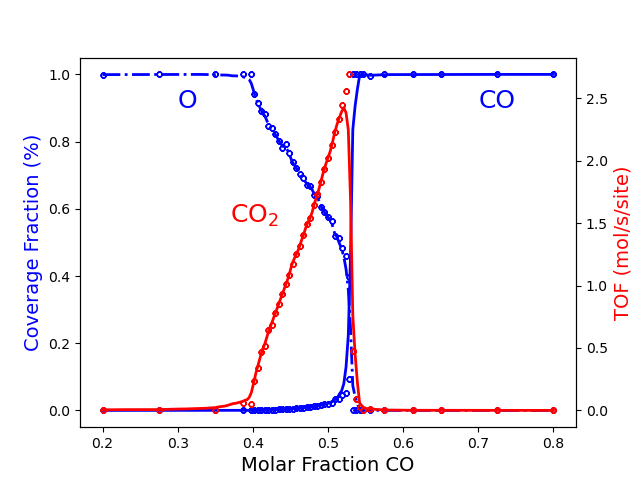
The above results are the final aim of the calculation. However, we can take advantage of python libraries to visualize them. Here, we use matplotlib. Please check the matplotlib documentation for more details at matplotlib. The following lines of code allow visualizing the effect of changing the \(CO\) molar fraction on the average coverage of \(O*\) and \(CO*\) and the production rate of \(CO_2\). In the Figure, we show the training data generated by the Zacros model as points and the Surrogate Model’s prediction as lines.
import matplotlib.pyplot as plt

fig = plt.figure()

x_CO_model = numpy.linspace(0.2, 0.8, 201)
ac_O_model, ac_CO_model, TOF_CO2_model = adpML.predict(x_CO_model).T

ax = plt.axes()
ax.set_xlabel("Molar Fraction CO", fontsize=14)

ax.set_ylabel("Coverage Fraction (%)", color="blue", fontsize=14)
ax.plot(x_CO_model, ac_O_model, color="blue", linestyle="-.", lw=2, zorder=1)
ax.plot(x_CO, ac_O, marker="$\u25EF$", color="blue", markersize=4, lw=0, zorder=1)
ax.plot(x_CO_model, ac_CO_model, color="blue", linestyle="-", lw=2, zorder=2)
ax.plot(x_CO, ac_CO, marker="$\u25EF$", color="blue", markersize=4, lw=0, zorder=1)
plt.text(0.3, 0.9, "O", fontsize=18, color="blue")
plt.text(0.7, 0.9, "CO", fontsize=18, color="blue")

ax2 = ax.twinx()
ax2.set_ylabel("TOF (mol/s/site)", color="red", fontsize=14)
ax2.plot(x_CO_model, TOF_CO2_model, color="red", linestyle="-", lw=2, zorder=0)
ax2.plot(x_CO, TOF_CO2, marker="$\u25EF$", color="red", markersize=4, lw=0, zorder=1)
plt.text(0.37, 1.5, "CO$_2$", fontsize=18, color="red")

plt.show()
We also found three regions involving the two phase transitions, as
shown in the Figure, which are similar to the ones obtained in the
example Phase Transitions in the ZGB model. However, as you can see,
the points are not equidistant here. The ADP generated more points for
\(x_\text{CO}\) between 0.35 and 0.55, which is likely to represent
the small oscillations that occur there accurately. It is worth noting
that the Surrogate Model has some difficulty reproducing the narrow peak
at a maximum \(CO_2\) TOF. Certainly, the model could perform
better. Unfortunately, the only way to do so is by increasing the number
of points in the training set by tuning the ADP parameters’
(algorithmParams). However, now that we have the surrogate model, we
can quickly obtain the average coverage for \(O*\) and \(CO*\)
and the \(CO_2\) TOF for any \(CO\) molar fraction.
Now, we can close the pyZacros environment:
scm.pyzacros.finish()
[02.02|22:52:41] PLAMS run finished. Goodbye
As a final note, you don’t have to recalculate any training points if
you load the surrogate model directly from the disk. As a result, you
can apply it to any other situation, such as e.g., a simulation of
reactive computational fluid dynamics (rCFD). The following code creates
the image above exactly, but it starts by reading the surrogate model
from the directory plams_workdir/adp.results/. It can be used in a
separate script.
import numpy as np
import adaptiveDesignProcedure as adp
import matplotlib.pyplot as plt

path = "plams_workdir/adp.results/"

x_CO_model = np.linspace(0.2, 0.8, 201)
ac_O_model, ac_CO_model, TOF_CO2_model = adp.predict(x_CO_model, path).T

ax = plt.axes()
ax.set_xlabel("Molar Fraction CO", fontsize=14)

ax.set_ylabel("Coverage Fraction (%)", color="blue", fontsize=14)
ax.plot(x_CO_model, ac_O_model, color="blue", linestyle="-.", lw=2, zorder=1)
ax.plot(x_CO_model, ac_CO_model, color="blue", linestyle="-", lw=2, zorder=2)
plt.text(0.3, 0.9, "O", fontsize=18, color="blue")
plt.text(0.7, 0.9, "CO", fontsize=18, color="blue")

ax2 = ax.twinx()
ax2.set_ylabel("TOF (mol/s/site)", color="red", fontsize=14)
ax2.plot(x_CO_model, TOF_CO2_model, color="red", linestyle="-", lw=2, zorder=0)
plt.text(0.37, 1.5, "CO$_2$", fontsize=18, color="red")

plt.show()
By default, the Surrogate Model’s file is ml_ExtraTrees_forCFD.pkl.
The option forestFile in the ADP constructor allows you to alter the
prefix ml_ExtraTrees. In the adp.predict() method, you can
provide the complete path to this file, but if a directory is supplied
instead, it will try to discover the proper file inside, as shown in the
lines of code above.
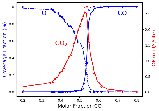
Model Refinement
We can alter the ADP parameters to perform a stricter optimization.
The dth and d2th parameters are refinement thresholds for the first and second derivatives calculated by the model. When large gradients are encountered in the training set, additional data is generated.
By lowering the dth and d2th thresholds, the resolution of the surrogate model can be improved.
Optimization parameters can be specified in the ADP settings. We update our script and re-start the calculation:
adpML = adp.adaptiveDesignProcedure( input_var, output_var, get_rate,
                                     algorithmParams={'dth':0.01,'d2th':0.10},
                                     outputDir=scm.pyzacros.workdir()+'/adp.results',
                                     randomState=10 )
This is seen to improve the replication of the narrow features:

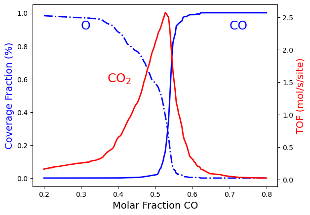
Steady-State Model
We can also perform the model fitting under steady-state conditions. The implementation is provided in the example script PhaseTransitions-SteadyState-ADP.py. We only had to update the get_rate() function to include the steady-state settings:
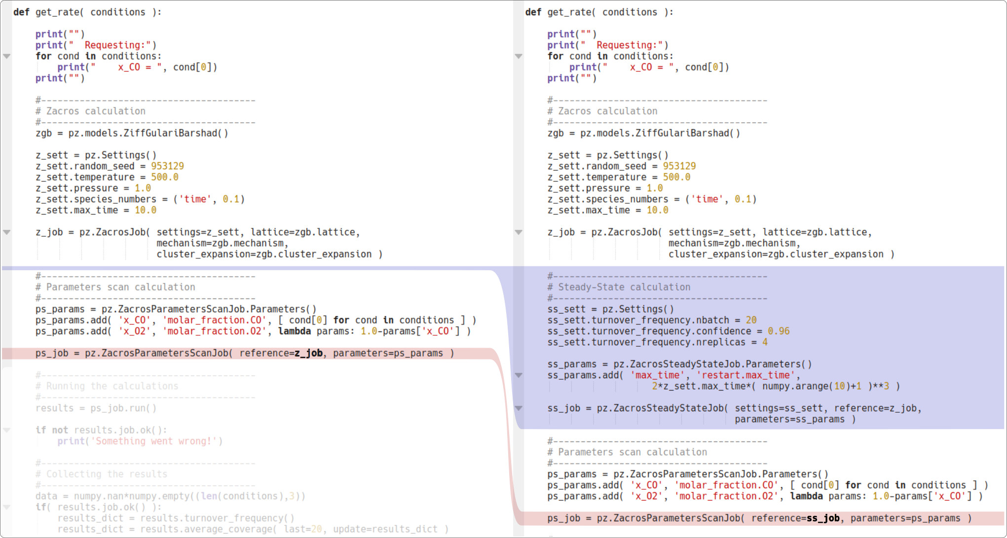
This calculation will take around 20 minutes to complete. Once it has finished, we obtain our surrogate model for the steady-state ZGB kinetics: