Setting up a QM/MM Simulation: a ‘Walk Thru’¶

Step 1. Partitioning the System and the Model QM system¶

First one must decide where to partition the system into QM and MM regions. This is actually a very important step since the partitioning can be considered the ‘original sin’. Much thought and testing should be put into deciding where to place the QM/MM boundary. In this example, we have chosen the partitioning depicted in Figure 5-1a in order to keep the example simple. In this figure the QM region enclosed in the dotted polygon, with two covalent bonds crossing the QM/MM boundary. One must also choose an appropriate QM model system for which the electronic structure calculation will be performed. To preserve the sp³ hybridization of the carbon center in the QM region, we must keep the carbon tetravalent. Thus, we will cap the two dangling bonds with dummy or capping hydrogen atoms. One can use any monovalent atom such as H or F, but H is probably best. The reason that monovalent atoms should be used for capping atoms is that one does not want capping atom to have any ‘dangling’ bonds. Capping or dummy groups can not be used. Figure 5-1b, depicts the QM model system with two capping hydrogen atoms. Thus, the electronic structure calculation will be performed on methane such that the capping hydrogen atoms lie along the bond vector of the link bond in the real system as shown in Figure 5-1b.

Figure 5-1 Cytocine QM/MM example model. a) Shows the whole system with the atoms enclosed in the dotted polygon making up the QM system. b) Shows the equivalent QM model system. The remainder of the cytocine molecule is shown ghosted to demonstrate the relationship between the model system and the full system. The QM model system consists of a closed shell methane molecule.

Step 2. Labeling of Atoms (QM, MM or LI)¶

Once a partitioning of the system has been established, one needs to designate each of the atoms in the full system as QM, LI or MM atom type. For the example system, these designations are shown in Figure 5-2a, where the atoms that are not labeled are MM atoms.

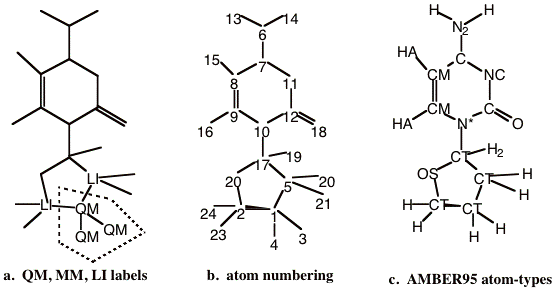
Figure 5-2 Labeling of the example model. a) QM, MM and LI designations. Atoms not labeled are ‘MM’ atoms. The dotted polygon encloses the QM region of the model. b) Atom numbering of the entire system. Note that the QM and LI atoms precede any MM atoms. c) The AMBER95 force field atom type designations.

All atoms within the dotted polygon are ‘QM’ type atoms. The atoms outside of the QM region will either be MM or LI atoms depending on whether they are part of a link bond or not. The covalent bonds that cross the QM/MM boundary are termed the link bonds. In the example system, there are two such covalent bonds. The atoms that lie on the MM side of the link bonds are labeled the LI atoms. Thus, these are all of the atoms that lie outside the dotted polygon that have a covalent bond to QM atoms. If there are no covalent bonds that traverse the QM/MM boundary, then there will be no LI atoms.

Step 3. Renumbering of Atoms¶

There is a strict rule concerning the ordering of the atoms, based on the QM, MM, or LI atom type designation. All QM and LI atoms must come before any MM atoms. A valid atom numbering for the example system is shown in figure 5-2b. Here the atoms labeled ‘QM’ or ‘LI’ in Figure 5-2a are the first five atoms of the molecular system.

Step 4. ADF QM/MM input: Atomic coordinates¶

Now we can begin to construct the input. We will begin with the atomic coordinates. For this example, we will optimize the geometry of the complex in Cartesian coordinates. Coordinates of the whole QM/MM complex or the ‘real’ complex should be defined here. DO NOT define the coordinates of the capping atoms. The program will calculate their positions, and add them automatically. The definition of the coordinates is done exactly as they are in a standard ADF run. Below is the ATOMS key block for our example system.

ATOMS Cartesian
  1 C  1.94807  3.58290 -0.58162
  2 C  1.94191  3.61595  1.09448
  3 H  1.69949  4.49893 -1.05273
  4 H  2.99455  3.17964 -0.86304
  5 C  0.94659  2.40054 -0.92364
  6 N -1.74397 -3.46417  0.31178
  7 C -1.00720 -2.20758  0.33536
  8 C -1.66928 -1.00652  0.31001
  9 C -0.92847  0.25653  0.34895
 10 N  0.43971  0.26735  0.38232
 11 N  0.36409 -2.20477  0.28992
 12 C  1.09714 -0.95413  0.22469
 13 H -2.89781 -3.50815  0.31746
 14 H -1.21484 -4.49217  0.31721
 15 H -2.80940 -0.93497  0.30550
 16 H -1.55324  1.21497  0.33885
 17 C  1.23309  1.44017  0.30994
 18 O  2.58277 -1.01636  0.23914
 19 H  2.37276  1.25557  0.29984
 20 O  1.02358  2.43085  1.50880
 21 H  1.17136  1.95097 -1.87367
 22 H -0.10600  2.77333 -0.80348
 23 H  1.62170  4.54039  1.51392
 24 H  2.99608  3.28749  1.41345
END

Step 5. Connection Table and MM force field types¶

In order to construct a molecular mechanics potential, the program needs to know the connectivity of the molecular system and the molecular mechanics force field atom-type designations. In this example we are using the AMBER95 force field of Kollman and coworkers [4]. The appropriate AMBER95 atom-types for this molecule are shown in Figure 5-2c. No new atom types need to be introduced to the standard AMBER95 force field to treat this system. However, if this were needed, then the force field file would have to be modified.

Next a connection table needs to be constructed. For this program this needs to be done on an atom by atom basis. Either a fully redundant connection table or a fully non-redundant connection table is acceptable. A redundant connection table refers to one in which the covalent bonds are defined for all atoms. For example, if X is bonded to Y, in the connections for atom X, a bond is defined to atom Y. For the connections to atom Y, a bond is also defined to atom X even though the bond has already been defined. In a non-redundant connection table, when a bond is defined in the connections for atom X, it is not again defined in the connections for atom Y.

We now can begin to construct part of the input, namely the MM_CONNECTION_TABLE subkey block of the QMMM key block. For this example, the MM_CONNECTION_TABLE key block is given below.

MM_CONNECTION_TABLE
 1 CT QM 2 3 4 5
 2 CT LI 1 20 23 24
 3 HC QM 1
 4 HC QM 1
 5 CT LI 1 17 21 22
 6 N2 MM 7 13 14
 7 CA MM 6 8 11
 8 CM MM 7 9 15
 9 CM MM 8 10 16
10 N* MM 9 12 17
11 NC MM 7 12
12 C MM 10 11 18
13 H MM 6
14 H MM 6
15 HA MM 8
16 H4 MM 9
17 CT MM 5 10 19 20
18 O MM 12
19 H2 MM 17
20 OS MM 2 17
21 HC MM 5
22 HC MM 5
23 H1 MM 2
24 H1 MM 2
SUBEND

The first column is simply the atom number. The atoms defined here MUST be in the same order as defined in the ATOMS key block provided in the previous section. Again, we do not include the capping atoms. The second column shows the AMBER95 atom-types for our system, displayed in Figure 5-2c. The third column is the MM, QM or LI designation. Notice that the QM and LI atoms appear before any MM atoms. The remaining columns are reserved for the connection table. In the above example, a fully redundant connection table is provided.

Step 6. LINK_BONDS¶

When there are covalent bonds that cross the QM/MM boundary, the LINK_BONDS subkey block is required. Since one only defines the ‘real system in both the ATOMS key block and the MM_CONNECTION_TABLE subkey block, this key block defines both the initial position of the capping atom and what kind of ADF fragment atom will be used as a capping atom. In this example we have two link bonds, both of which will be ‘capped’ with capping hydrogen atoms as shown in Figure 5-1b. Below is the LINK_BONDS subkey block for our example.

LINK_BONDS
  1 - 5 1.380 H
  1 - 2 1.375 H
SUBEND

The first part of the input specifies the atoms involved in link bonds. Here QM atom 1 forms link bonds with atoms 5 and 2. The column in the input is the link bond a parameter, which is defined as the ratio between the capping bond length in the QM model system and the bond length of the corresponding link bond in the real system. This ratio can be determined by taking the necessary bond lengths from a pure QM calculation of the model QM system, and the bond length from the whole complex. If those are not available, they can be taken from tabulated bond lengths or bond lengths of similar bonds in other complexes. There is an independent a parameter for each link bond. It is VERY IMPORTANT to emphasize that the total energy of the QM/M system is dependent upon the a parameters. Thus, if one is comparing the energetics of two conformational isomers calculated with the QM/MM method, this comparison is only valid if the a parameters used are the same. In our example, ratios of 1.38 and 1.375 were used. This is somewhat typical ratio of C-H to C-C bond lengths, in aliphatic hydrocarbons. The last column in the LINK_BONDS input refers to the ADF fragment for which will be used for the capping atom in the electronic structure calculation. Please, note this fragment must be present in the FRAGMENTS key block of the ADF input.

Step 7. Assignment of Atomic Charges¶

Perhaps the most dubious aspect of the QM/MM approach involves the non-bonded electrostatic interaction between the QM and MM regions. The ADF QM/MM extension currently only supports placement of static point charges on MM atoms. At the moment, you have two options. First, you can chose to have the MM point charges to interact with the electron density of the QM model system, thereby allowing the wave function of the QM system to be polarized. Alternatively, you can assign static point charges to the QM atoms which interact with MM point charges as would happen if the whole system were treated with a molecular mechanics force field. In this example, we will choose the latter, using the standard AMBER95 charges cytosine. To specific how the electrostatic interactions between the two regions are treated, one uses the ELSTAT_COUPLING_MODEL keyword in the QMMM key block and sets it equal to 1.

In ADF QM/MM the atomic point charges can be assigned on an atom-type basis, where the point charges are taken from the force field file. It can also be defined on a per atom basis, where a unique charge is assigned to each atom in the molecular system in the CHARGES subkey block. Since the charges in AMBER95 are assigned according to the nucleic or amino acid, we must assign the charges on a per-atom basis. Given below is the CHARGES subkey block with the appropriate AMBER95 point charges assigned to the system. The first column in this subkey block is the atom numbering. It is important to use the right atom number instead because the program actually determines the charges on each atom individually by searching for the atom number within this key block. Charges don’t have to be in order.

ELSTAT_COUPLING_MODEL=1
CHARGES
 1 0.0000
 2 0.0000
 3 0.0000
 4 0.0000
 5 0.0000
 6 -0.9530
 7 0.8185
 8 -0.5215
 9 0.0053
 10 -0.0484
 11 -0.7584
 12 0.7538
 13 0.4234
 14 0.4234
 15 0.1928
 16 0.1958
 17 0.0066
 18 -0.6252
 19 0.2902
 20 -0.2033
 21 0.0000
 22 0.0000
 23 0.0000
 24 0.0000
SUBEND

Step 8. Remainder of the QMMM key block¶

The ADF QM/MM input is almost complete. Now only a few settings need to be defined in the QMMM key block. The remainder of the QMMM key block is given below.

FORCEFIELD_FILE /usr/bob/QMMM_data/amber95.ff
RESTART_FILE mm.restart
OUTPUT_LEVEL=1
WARNING_LEVEL=2

The FORCEFIELD_FILE defines the filename of the force field file to be used. If the force field file is not in the running directory of the ADF job, then the full path needs to be specified. The RESTART_FILE specifies the name of the QM/MM restart to be written. If the job is a restart itself, this keyword also specifies the QM/MM restart file to read.

The OUTPUT_LEVEL specifies how much output to print during the course of the ADF QM/MM run. OUTPUT_LEVEL=1 is good for most purposes. Using an OUTPUT_LEVEL=2 is good when trouble shooting, but probably provides too much output when the job is running normally. The WARNING_LEVEL keyword specifies when to stop the job. When it is set to 2, the run stops at any spot where a potential QM/MM problem is detected. This is good when first setting up a job because the program attempts to point out potential problems.

Step 9. Putting it all together: The whole ADF QM/MM input¶

The whole ADF QM/MM input for the sample system is given below. The following will be a QM/MM geometry optimization performed in Cartesian coordinates with no constraints. Some comments are provided in bold.

Title CYT amber95 test - CARTESIAN GEOMETRY OPTIMIZATION NO CONSTRAINTS
Fragments
 C T21.C.III.1s            ! Notice that only fragments for the calculation of
 H T21.H.III               ! model system are needed.
End

Symmetry NOSYM

Charge 0 0                 ! This refers to the charge of the QM model system, not the 'real' system

ATOMS Cartesian
 1 C 1.94807 3.58290 -0.58162
 2 C 1.94191 3.61595 1.09448
 3 H 1.69949 4.49893 -1.05273
 4 H 2.99455 3.17964 -0.86304
 5 C 0.94659 2.40054 -0.92364
 6 N -1.74397 -3.46417 0.31178
 7 C -1.00720 -2.20758 0.33536
 8 C -1.66928 -1.00652 0.31001
 9 C -0.92847 0.25653 0.34895
 10 N 0.43971 0.26735 0.38232
 11 N 0.36409 -2.20477 0.28992
 12 C 1.09714 -0.95413 0.22469
 13 H -2.89781 -3.50815 0.31746
 14 H -1.21484 -4.49217 0.31721
 15 H -2.80940 -0.93497 0.30550
 16 H -1.55324 1.21497 0.33885
 17 C 1.23309 1.44017 0.30994
 18 O 2.58277 -1.01636 0.23914
 19 H 2.37276 1.25557 0.29984
 20 O 1.02358 2.43085 1.50880
 21 H 1.17136 1.95097 -1.87367
 22 H -0.10600 2.77333 -0.80348
 23 H 1.62170 4.54039 1.51392
 24 H 2.99608 3.28749 1.41345
END

QMMM
 FORCEFIELD_FILE amber95.ff
 RESTART_FILE mm.restart
 OUTPUT_LEVEL=1
 WARNING_LEVEL=2
 ELSTAT_COUPLING_MODEL=1
 LINK_BONDS
   1 - 5 1.38000 H
   1 - 2 1.38030 H
 SUBEND
 MM_CONNECTION_TABLE
   1 CT QM 2 3 4 5
   2 CT LI 1 20 23 24
   3 HC QM 1
   4 HC QM 1
   5 CT LI 1 17 21 22
   6 N2 MM 7 13 14
   7 CA MM 6 8 11
   8 CM MM 7 9 15
   9 CM MM 8 10 16
   10 N* MM 9 12 17
   11 NC MM 7 12
   12 C MM 10 11 18
   13 H MM 6
   14 H MM 6
   15 HA MM 8
   16 H4 MM 9
   17 CT MM 5 10 19 20
   18 O MM 12
   19 H2 MM 17
   20 OS MM 2 17
   21 HC MM 5
   22 HC MM 5
   23 H1 MM 2
   24 H1 MM 2
 SUBEND
 CHARGES
   1 0.0 CT
   2 0.0 CT
   3 0.0 HC
   4 0.0 HC
   5 0.0 CT
   6 -0.9530 N2
   7 0.8185 CA
   8 -0.5215 CM
   9 0.0053 CM
   10 -0.0484 N*
   11 -0.7584 NC
   12 0.7538 C
   13 0.4234 H
   14 0.4234 H
   15 0.1928 HA
   16 0.1958 H4
   17 0.0066 CT
   18 -0.6252 O
   19 0.2902 H2
   20 -0.2033 OS
   21 0.0000 HC
   22 0.0000 HC
   23 0.0000 H1
   24 0.0000 H1
 SUBEND
END

GEOMETRY
 ITERATIONS 20
 CONVERGE E=1.0E-3 GRAD=0.0005
 STEP RAD=0.3 ANGLE=5.0
 DIIS N=5 OK=0.1 CYC=3
END

XC
 LDA VWN
 GGA POSTSCF Becke Perdew
End

Integration 3.0

SCF
 Iterations 60
 Converge 1.0E-06 1.0E-6
 Mixing 0.20
 DIIS N=10 OK=0.500 CX=5.00 CXX=25.00 BFAC=0.00
End

End Input

In the above example, the geometry was defined with Cartesian coordinates and the geometry optimization was also done in Cartesians. The same input could also have easily been defined with a Z-matrix in the ATOMS key block.

Step 1. Partitioning the System and the Model QM system.¶

First one must decide where to partition the system into QM and MM regions. For this example, we have decide to partition the system as illustrated in Figure 53b, whereby the QM region is contained in the dotted polygon. The corresponding QM model system, for which the electronic structure calculation will be performed, is depicted in Figure 5-3b. In the model QM system the link atoms have been replaced by capping hydrogen atoms. Notice that the QM/MM boundary cuts through the cyclopentadienyl ring of the ferrocenyl ligand. Based on experimental studies of this complex, it is assumed that the ferrocenyl ligand acts only as a spectator ligand and can be modeled effectively on a steric basis only. Using an olefinic group will approximate the sp2 hybridization of the Cp rings. Here, special care must be taken to preserver the structural features of the Cp ring. For example the C-C bond distance in the ferrocenyl ligand is approximately 1.45 Ang whereas it is about 1.34 Ang in an olefin. This will be elaborated on later. The replacement of the phenyl phosphine in the real system by hydrogen phosphine will have some consequences due to the different electronic properties of the substituents. It is known that the phenyl substitution on the phosphine is more electron withdrawing than the hydrogen substituent. The replacement of the phenyl phosphine with hydrogen phosphine will result in a contraction of the Pd-P bond in the QM model system and hence the Pd-P bond will be too short in our QM/MM model.

Step 2. Labeling of Atoms¶

Once a partitioning of the system has been established, one needs to label each of the atoms in the full system as QM, LI or MM atom type. For the example system, all atoms contained within the dotted polygon in Figure 5-3a are ‘QM’ atoms. All atoms that are marked with asterisks in Figure 5-3a are ‘LI’ atoms and finally the remaining atoms outside the dotted polygon are ‘MM’ atoms. The dummy atom that we need in order to define our reaction coordinate is designated a QM atom. This dummy atom will be made to lie midway between the two olefinic carbon atoms of the ethene moiety. It is important to realize that the linear transit constraint cannot involve any MM atoms. Two dummy atoms representing the center of the Cp rings of the ferrocenyl ligand will also be introduced. They we be part of the MM subsystem.

Step 3. Renumbering of Atoms¶

It will be re-emphasize that there is a strict rule concerning the ordering of the atoms, based on their QM, MM, or LI atom type designation. All QM and LI atoms must come before any MM atoms. This rule also applies to the dummy atoms. All atoms in the QM model system shown in Figure 5-3b and their equivalent LI atoms in the real system must come first. Given below are the Cartesian coordinates of the initial geometry with the atoms renumbered. Although the optimization will be performed in internal coordinates, this is a complex example, and it might help the reader to examine the 3D structure of the complex with their favorite molecule viewer.

Pd 0.00000 0.00000 0.00000
N 2.18381 0.00000 0.00000
P -0.19353 2.33087 0.00000
Si -2.09382 -0.72920 0.40993
Cl -3.11786 -1.66043 -1.19030
Cl -3.49847 0.77293 1.00006
Cl -2.26795 -2.09058 2.02296
C 1.00751 3.35326 -0.90266
C 2.19320 2.92863 -1.63738
C 2.55933 1.49397 -1.90948
N 3.04680 0.78384 -0.70880
C 4.30216 0.71267 -0.18548
C 4.25805 -0.16196 0.88628
C 2.91893 -0.57760 0.96569
Xx 0.74788 -1.69468 -1.67891
C 1.00986 -2.06361 -1.18981
C 0.48590 -1.32574 -2.16801
H 0.42486 -2.82737 -0.67948
H 2.04440 -1.93825 -0.86750
H 1.06712 -0.55943 -2.68284
H -0.54392 -1.46716 -2.49409
C -0.02313 3.09172 1.69751
C -1.80681 3.04317 -0.56800
C 1.06326 4.78500 -0.83878
C 2.90531 4.10963 -2.00851
H 1.82015 0.84892 -1.41063
C 2.56571 1.10455 -3.38246
H 5.13150 1.27389 -0.59600
H 5.08293 -0.44584 1.52605
C 2.28008 -1.58274 1.88382
Fe 1.04114 4.20972 -2.75447
H 3.29128 1.69565 -3.95722
H 2.82573 0.03883 -3.48724
H 1.57260 1.26129 -3.82619
C 2.23262 5.27491 -1.51096
H 3.82950 4.13635 -2.57654
H 2.53722 6.31008 -1.62736
H 0.35288 5.41923 -0.32204
C -0.36634 3.33949 -3.93243
C -0.80398 4.62382 -3.46691
C 0.14944 5.60144 -3.90508
C 1.17457 4.92275 -4.64218
C 0.85084 3.52607 -4.66695
H 1.38331 2.75840 -5.21594
H -0.88905 2.39926 -3.80335
H -1.70862 4.82843 -2.90699
H 0.10418 6.66814 -3.70967
H 2.03573 5.38561 -5.11158
C -2.52881 2.31699 -1.52071
C -3.74190 2.80302 -2.01422
C -4.24163 4.02394 -1.55340
C -3.52216 4.75609 -0.60549
C -2.30668 4.26891 -0.11529
H -2.14465 1.36750 -1.87729
H -4.29443 2.23258 -2.75379
H -5.18572 4.40286 -1.93263
H -3.90891 5.70542 -0.24710
H -1.76468 4.85404 0.61704
C -1.11030 3.12908 2.57588
C -0.97634 3.68572 3.85061
C 0.25426 4.20707 4.25852
C 1.35020 4.15676 3.39277
C 1.21425 3.58782 2.12359
H -2.06730 2.72549 2.27375
H -1.82678 3.71355 4.52356
H 0.35921 4.64813 5.24539
H 2.30826 4.55806 3.70733
H 2.08227 3.52803 1.47710
C 2.71278 -2.91472 1.84328
C 2.09262 -3.86832 2.66014
C 1.02394 -3.51226 3.48850
C 0.62539 -2.17333 3.54762
C 1.26348 -1.20208 2.77018
C 3.85077 -3.34061 0.90256
H 2.44054 -4.89548 2.65117
C 0.28665 -4.56067 4.32981
H -0.18696 -1.88618 4.20708
C 0.83254 0.25922 2.93922
H 4.81150 -3.02160 1.33267
H 3.72469 -2.87842 -0.08835
H 3.87528 -4.43158 0.76399
H 1.55468 0.95128 2.48757
H 0.75353 0.50536 4.00860
H -0.15276 0.39937 2.47265
H -0.79950 -4.40165 4.25848
H 0.51050 -5.58360 3.99174
H 0.59686 -4.45719 5.38063
Xx 1.88038 4.09028 -1.37966
Xx 0.20091 4.40271 -4.12271

Step 4. Z-matrix and constraints¶

This simulation will be a linear transit simulation where the reaction coordinate will be the distance from the Pd center to the midpoint of the complexed ethene molecule. In order to use midpoint of the ethene molecule as the reaction coordinate we must use a dummy atom to define the midpoint and a few constraints to maintain the dummy atom at the midpoint. The dummy atom is atom number 15 and the two carbon atoms of the ethene moiety are atoms 16 and 17. Each of the two carbons of the ethene will be ‘bonded’ to the midpoint using the same (free) bond distance variable ‘B15’. This will ensure that the midpoint dummy atom is always equidistant to each ethene carbon. To ensure that the midpoint dummy atom always lies along the C-C bond vector the dihedral variable ‘D14’ will be constrained to 180 degrees. Finally, to prevent C-C bond distance of olefinic group used to model the ferrocenyl ligand to revert to its natural bond length of approximately 1.34 Ang, the C-C distance (B8) will be constrained to 1.45 Ang. This is the distance found in the C-C bond distance in the ferrocenyl ligand. One might be concerned about the internal coordinate definition of the cyclopentadienyl rings of the ferrocenyl ligand. Since the ferrocenyl ligand is part of the MM region, the Z-matrix will be used only to construct the initial geometry. From there the molecular mechanics borderleft takes over and where the optimization is done in Cartesian coordinates. For MM atoms it is important that care be taken when defining the connection table.

ATOMS internal
 Pd 0 0 0 0 0 0
 N 1 0 0 B1 0 0
 P 1 2 0 B2 A1 0
 Si 1 2 3 B3 A2 D1
 Cl 4 1 2 B4 A3 D2
 Cl 4 1 5 B5 A4 D3
 Cl 4 1 5 B6 A5 D4
 C 3 1 2 B7 A6 D5
 C 8 3 1 B8 A7 D6
 C 9 8 3 B9 A8 D7
 N 10 9 8 B10 A9 D8
 C 11 2 1 B11 A10 D9
 C 12 11 2 B12 A11 D10
 C 2 1 11 B13 A12 D11
 XX 1 2 3 B14 A13 D12
 C 15 1 2 B15 A14 D13
 C 15 1 16 B15 A15 D14
 H 16 15 1 B17 A16 D15
 H 16 17 18 B18 A17 D16
 H 17 16 18 B19 A18 D17
 H 17 16 18 B20 A19 D18
 C 3 1 8 B21 A20 D19
 C 3 1 8 B22 A21 D20
 C 8 3 9 B23 A22 D21
 C 9 8 10 B24 A23 D22
 H 10 9 8 B25 A24 D23
 C 10 9 26 B26 A25 D24
 H 12 11 13 B27 A26 D25
 H 13 12 11 B28 A27 D26
 C 14 2 1 B29 A28 D27
 Fe 24 8 3 B30 A29 D28
 H 27 10 9 B31 A30 D29
 H 27 10 32 B32 A31 D30
 H 27 10 32 B33 A32 D31
 C 25 9 8 B34 A33 D32
 H 25 9 35 B35 A34 D33
 H 35 25 9 B36 A35 D34
 H 24 8 31 B37 A36 D35
 C 31 24 8 B38 A37 D36
 C 39 31 24 B39 A38 D37
 C 40 39 31 B40 A39 D38
 C 41 40 39 B41 A40 D39
 C 39 31 40 B42 A41 D40
 H 43 39 31 B43 A42 D41
 H 39 31 40 B44 A43 D42
 H 40 39 41 B45 A44 D43
 H 41 40 42 B46 A45 D44
 H 42 41 40 B47 A46 D45
 C 23 3 1 B48 A47 D46
 C 49 23 3 B49 A48 D47
 C 50 49 23 B50 A49 D48
 C 51 50 49 B51 A50 D49
 C 52 51 50 B52 A51 D50
 H 49 23 50 B53 A52 D51
 H 50 49 51 B54 A53 D52
 H 51 50 52 B55 A54 D53
 H 52 51 53 B56 A55 D54
 H 53 52 51 B57 A56 D55
 C 22 3 1 B58 A57 D56
 C 59 22 3 B59 A58 D57
 C 60 59 22 B60 A59 D58
 C 61 60 59 B61 A60 D59
 C 62 61 60 B62 A61 D60
 H 59 22 60 B63 A62 D61
 H 60 59 61 B64 A63 D62
 H 61 60 62 B65 A64 D63
 H 62 61 63 B66 A65 D64
 H 63 62 61 B67 A66 D65
 C 30 14 2 B68 A67 D66
 C 69 30 14 B69 A68 D67
 C 70 69 30 B70 A69 D68
 C 71 70 69 B71 A70 D69
 C 72 71 70 B72 A71 D70
 C 69 30 70 B73 A72 D71
 H 70 69 71 B74 A73 D72
 C 71 70 72 B75 A74 D73
 H 72 71 73 B76 A75 D74
 C 73 72 71 B77 A76 D75
 H 74 69 30 B78 A77 D76
 H 74 69 79 B79 A78 D77
 H 74 69 79 B80 A79 D78
 H 78 73 72 B81 A80 D79
 H 78 73 82 B82 A81 D80
 H 78 73 82 B83 A82 D81
 H 76 71 70 B84 A83 D82
 H 76 71 85 B85 A84 D83
 H 76 71 85 B86 A85 D84
 XX 24 8 31 B87 A86 D85
 XX 41 40 42 B88 A87 D86
END

GEOVAR
 B1=2.18381
 B2=2.33889
 B3=2.25474
 B4=2.11579
 B5=2.13955
 B6=2.11791
 B7=1.81730
 B8=1.45807 F
 B9=1.50544
 B10=1.47768
 B11=1.36193
 B12=1.38405
 B13=1.34409
 B14=2.50000 5.000
 B15=0.66631
 B17=1.08903
 B18=1.09082
 B19=1.09092
 B20=1.08943
 B21=1.86801
 B22=1.85275
 B23=1.43426
 B24=1.42814
 B25=1.10060
 B26=1.52360
 B27=1.08226
 B28=1.08182
 B29=1.50380
 B30=2.00032
 B31=1.09827
 B32=1.10198
 B33=1.09896
 B34=1.43456
 B35=1.08513
 B36=1.08532
 B37=1.08347
 B38=2.03122
 B39=1.43448
 B40=1.43413
 B41=1.43347
 B42=1.43383
 B43=1.08361
 B44=1.08347
 B45=1.08341
 B46=1.08540
 B47=1.08451
 B48=1.39867
 B49=1.39691
 B50=1.39740
 B51=1.39722
 B52=1.39822
 B53=1.08455
 B54=1.08520
 B55=1.08569
 B56=1.08594
 B57=1.08280
 B58=1.39816
 B59=1.39740
 B60=1.39734
 B61=1.39754
 B62=1.39750
 B63=1.08166
 B64=1.08484
 B65=1.08604
 B66=1.08530
 B67=1.08396
 B68=1.40109
 B69=1.40042
 B70=1.39823
 B71=1.39824
 B72=1.39818
 B73=1.53667
 B74=1.08452
 B75=1.53315
 B76=1.08501
 B77=1.53287
 B78=1.09990
 B79=1.10064
 B80=1.10001
 B81=1.09746
 B82=1.10018
 B83=1.09915
 B84=1.10005
 B85=1.10036
 B86=1.10053
 B87=1.20119
 B88=1.21941
 A1=94.7463
 A2=158.2223
 A3=117.0192
 A4=115.6423
 A5=115.0054
 A6=120.3960
 A7=128.6001
 A8=124.4982
 A9=113.0381
 A10=110.6944
 A11=107.5291
 A12=123.1566
 A13=72.5934
 A14=90.0001
 A15=90.0001
 A16=121.4060
 A17=121.7463
 A18=121.7273
 A19=121.2990
 A20=113.4758
 A21=117.0770
 A22=124.4140
 A23=107.1936
 A24=108.2564
 A25=114.7923
 A26=122.2418
 A27=126.8321
 A28=119.5733
 A29=70.7204
 A30=111.7865
 A31=109.8825
 A32=110.4946
 A33=110.3514
 A34=125.5260
 A35=127.2980
 A36=125.4579
 A37=133.3349
 A38=68.8766
 A39=107.9605
 A40=108.0463
 A41=69.7028
 A42=125.7664
 A43=129.5676
 A44=126.2672
 A45=125.9595
 A46=126.0404
 A47=117.3031
 A48=120.5489
 A49=119.8703
 A50=119.8287
 A51=120.1922
 A52=119.7123
 A53=120.0017
 A54=120.0478
 A55=119.9075
 A56=118.9447
 A57=120.7197
 A58=120.6090
 A59=119.9563
 A60=119.7586
 A61=120.0640
 A62=120.1660
 A63=120.0615
 A64=120.1253
 A65=119.9602
 A66=119.0914
 A67=119.1156
 A68=119.5849
 A69=120.7057
 A70=119.1275
 A71=120.7701
 A72=120.6568
 A73=119.8697
 A74=121.2330
 A75=119.5074
 A76=118.2033
 A77=109.0914
 A78=110.4834
 A79=111.6228
 A80=111.7639
 A81=109.9169
 A82=109.0716
 A83=109.9009
 A84=111.6715
 A85=108.9122
 A86=55.1829
 A87=54.0180
 D1=-150.6568
 D2=-100.8347
 D3=-119.5809
 D4=123.4778
 D5=35.1598
 D6=-2.9958
 D7=7.2171
 D8=-72.9107
 D9=164.5027
 D10=0.9220
 D11=163.0063
 D12=135.2677
 D13=65.6662
 D14=180.0000 F
 D15=90.0000
 D16=179.5031
 D17=-179.9904
 D18=-0.4168
 D19=-117.3520
 D20=124.7005
 D21=-169.6021
 D22=-179.2713
 D23=-3.3919
 D24=119.3500
 D25=179.9891
 D26=-179.9514
 D27=17.4102
 D28=-129.2972
 D29=60.6432
 D30=120.3390
 D31=-120.3043
 D32=1.2969
 D33=179.4155
 D34=179.5397
 D35=123.6746
 D36=68.3005
 D37=62.0893
 D38=58.4426
 D39=0.0736
 D40=119.7199
 D41=127.1496
 D42=-120.1862
 D43=178.4186
 D44=-179.8093
 D45=179.5019
 D46=-30.2454
 D47=-178.8402
 D48=-0.0598
 D49=0.3012
 D50=-0.1575
 D51=-179.8476
 D52=-179.9824
 D53=179.8951
 D54=-179.8926
 D55=179.8489
 D56=-81.7949
 D57=179.3002
 D58=-0.2287
 D59=-0.6445
 D60=0.0510
 D61=-179.9960
 D62=179.9913
 D63=-179.8879
 D64=-179.8700
 D65=-178.0390
 D66=114.6178
 D67=-177.7647
 D68=1.7082
 D69=-3.4460
 D70=1.3564
 D71=179.4189
 D72=179.8505
 D73=-179.9397
 D74=-179.8352
 D75=-176.6101
 D76=76.9134
 D77=-120.1615
 D78=119.9038
 D79=165.3767
 D80=-119.6911
 D81=121.2928
 D82=-135.8162
 D83=120.3122
 D84=-119.4211
 D85=-58.7928
 D86=0.0762
END

Step 5. Connection Table, MM force field atom-types and Force Field Modification¶

In order to construct a molecular mechanics potential, the program needs to know the connectivity of the molecular system and the molecular mechanics force field atom-type designations. In this example we are using the Tripos or Sybyl force field. The Tripos force field does not support either Pd or ferrocenyl ligands, so we need to modify the standard force field file to handle these groups. Modification of a molecular mechanics force field without re-parameterization of the force field may not always be appropriate. However, in this case sort of ‘ad hoc’ additions to the Tripos force field can be justified. For Pd, all of the principle interactions will be contained within the QM region and only weak non-bonded interactions involving Pd will be approximated by the molecular mechanics potential. The ferrocenyl ligand is assumed to act as a spectator ligand and therefore it is adequate to simply attain the approximate structure of the complex with the molecular mechanics potential.

In the Tripos force field, the nitrogen atoms of the pyrazole ring should be assigned the ‘N_2’ atom-type; the P atom of the phosphine should be assigned the ‘P_3’ atom-type. The Cl, H and Si atoms are given the ‘Cl’, ‘H’, and ‘Si’ atom types respectively. The carbon atoms of the phenyl substituents are given the ‘C_ar’ atom-type, while the sp³ hybridized carbon atoms are given the ‘C_3’ atom-type.

Connections involving the dummy atom defining the midpoint of the ethene molecule are really not needed since this atom is contained within the QM region.

For the ferrocenyl ligand the ferrocene force field of Bosnich and coworkers will be used. Four new MM atom types will be introduced, C_cp, H_cp and CEN, representing the carbon, hydrogen and centroid of the cyclopentadienyl rings, respectively and Fe. In the connection table, the C_cp atoms will be bonded to the centroid and not the Fe center. The only two bonds made to the Fe center will be to the (two) central dummy atoms of the Cp rings. In making a connection between the C_cp atom and the centroid, a direct bond will is made to a QM atom and a MM atom. A warning will be issued during the run but as long as the ‘WARNING_LEVEL’ flag is set to 1 the job will continue. In this case the link bond between the C_cp atom and the centroid does not need to be mediated by a capping atom. This bond is used only for the construction of the MM potential for the ferrocenyl ligand. Special bond stretching, bending, torsion and out-of-plane potentials need to be added to the force field file. For the most part these parameters are taken from the Bosnich Ferrocene force field. For example for the bond stretches, the following potentials need to be added to the force field.

# Parameters added for Pd - ethene complex
C_cp C_cp 1  1400.00 1.434   From the Bosnich ferrocene force field.
C_cp H_cp 1   692.00 1.085   Bosnich
CEN  Fe   1   600.00 1.617   Bosnich
CEN  C_cp 1   600.00 1.220   Bosnich

The force field file is simply a text file and so the above section needs to be added to the ‘BONDS’ key block between the two ‘=======’ separator lines. Bond potentials need to be defined between the centroid of the Cp rings with the Fe center and the carbon atoms.

For the angle and torsion terms, the additions are somewhat more complex. The following angle potential terms need to be introduced.

# Parameters added for Pd - ethene complex
C_cp  C_cp  C_cp  1  78.80  126.0   Bosnich
C_cp  C_cp  H_cp  1  78.80  126.0   Bosnich
CEN   C_cp  C_cp  1   0.00    0.0   no potential
CEN   C_cp  H_cp  1   0.00    0.0   no potential
C_cp  CEN   C_cp  1   0.00    0.0   no potential
C_cp  CEN   Fe    1 100.00   90.0   Bosnich
CEN   Fe    CEN   1 100.00  180.0   Bosnich
CEN   C_cp  P_3   1   0.00    0.0   no potential
CEN   C_cp  C_3   1   0.00    0.0   no potential

Any angle potentials involving the Cp centroid and any atoms outside of the ferrocenyl ligand have been set to zero since the centroid was only a construct for the optimization of the ferrocenyl ligand. For the torsions, the following potentials have been added to the standard Tripos force field.

# Parameters added for Pd - ethene complex
P_3   C_cp  C_cp  C_cp  2   2.0000  -2.0  Sybyl *-C_ar-C_ar-* aromatic bond
P_3   C_cp  C_cp  H_cp  2   2.0000  -2.0  Sybyl *-C_ar-C_ar-* aromatic bond
C_3   C_cp  C_cp  H_cp  2   2.0000  -2.0  Sybyl *-C_ar-C_ar-* aromatic bond
H_cp  C_cp  C_cp  H_cp  2   2.0000  -2.0  Sybyl *-C_ar-C_ar-* aromatic bond
*     C_cp  C_cp  C_cp  2   2.3500  -2.0  same as SYBYL * C_ar C_ar C_ar
*     Fe    CEN   *     0   0.0000  -2.0  no potential involving centroid
*     C_cp  CEN   *     0   0.0000   0.0  no potential involving centroid
*     C_cp  C_cp  CEN   0   0.0000   0.0  no potential involving centroid
Pd    P_3   C_cp  CEN   0   0.0000   0.0  no potential involving centroid
CEN   C_cp  P_3   C_ar  0   0.0000   0.0  no potential involving centroid
N_2   C_3   C_cp  CEN   0   0.0000   0.0  no potential involving centroid
CEN   C_cp  C_3   H     0   0.0000   0.0  no potential involving centroid
CEN   C_cp  C_3   C_3   0   0.0000   0.0  no potential involving centroid

Here any torsional potentials involving the Centroid atom of the ferrocenyl ligand were set to zero. Torsional potentials involving atoms outside of the ferrocenyl ligand and having the C_cp-C_cp atoms central atom pair, these potentials were equated with those of the Tripos ‘ *-C_ar C_ar - * ‘ torsional potentials. Again, these somewhat arbitrary choices for the MM potentials involving the ferrocenyl ligand are justified by the fact that the ferrocenyl ligand acts only as a spectator group.

The van der Waals parameters used for the five new atoms types, Pd, Fe, CEN, C_cp and H_cp were taken from either existing Tripos van der Waals parameters of similar atom-types or they were taken from Rappe’s UFF (Universal Force Field). They are given below with their origins provided in the ‘NOTES’ column.

# Parameters added for Pd - ethene complex
C_cp  0.1070  3.4000  12.00 same as Tripos C_ar
Fe    0.0130  2.9120  12.00 UFF92 Fe6+2
Pd    0.0480  2.8990  12.00 UFF92 Pd4+2
CEN   0.0000  1.0000  12.00 zero
H_cp  0.0420  3.0000  12.00 same as Tripos H

Now that the addition of the new MM potentials and atom-types has been discussed, the ‘MM_CONNECTION_TABLE’ subkey block is given below. In practice, one typically constructs the input first, and then runs the program to see what force field potentials/parameters are missing. If any force field parameters are missing in the force field file, the ADF QM/MM program will print all missing potentials that need to be defined in the force field and then stop.

MM_CONNECTION_TABLE
 1 Pd QM 2 3 4 0 0 0
 2 N_2 QM 1 11 14 0 0 0
 3 P_3 QM 1 8 22 23 0 0
 4 Si QM 1 5 6 7 0 0
 5 Cl QM 4 0 0 0 0 0
 6 Cl QM 4 0 0 0 0 0
 7 Cl QM 4 0 0 0 0 0
 8 C_cp QM 3 9 24 88 0 0
 9 C_cp QM 8 10 25 88 0 0
 10 C_3 QM 9 11 26 27 0 0
 11 N_2 QM 2 10 12 0 0 0
 12 C_ar QM 11 13 28 0 0 0
 13 C_ar QM 12 14 29 0 0 0
 14 C_ar QM 2 13 30 0 0 0
 15 XX QM 16 17 1 0 0 0
 16 C_2 QM 15 17 18 19 0 0
 17 C_2 QM 15 16 20 21 0 0
 18 H QM 16 0 0 0 0 0
 19 H QM 16 0 0 0 0 0
 20 H QM 17 0 0 0 0 0
 21 H QM 17 0 0 0 0 0
 22 C_ar LI 3 59 63 0 0 0
 23 C_ar LI 3 49 53 0 0 0
 24 C_cp LI 8 35 38 88 0 0
 25 C_cp LI 9 35 36 88 0 0
 26 H QM 10 0 0 0 0 0
 27 C_3 LI 10 32 33 34 0 0
 28 H QM 12 0 0 0 0 0
 29 H QM 13 0 0 0 0 0
 30 C_ar LI 14 69 73 0 0 0
 31 Fe MM 88 89 0 0 0 0
 32 H MM 27 0 0 0 0 0
 33 H MM 27 0 0 0 0 0
 34 H MM 27 0 0 0 0 0
 35 C_cp MM 24 25 37 88 0 0
 36 H_cp MM 25 0 0 0 0 0
 37 H_cp MM 35 0 0 0 0 0
 38 H_cp MM 24 0 0 0 0 0
 39 C_cp MM 40 43 45 89 0 0
 40 C_cp MM 39 41 46 89 0 0
 41 C_cp MM 40 42 47 89 0 0
 42 C_cp MM 41 43 48 89 0 0
 43 C_cp MM 39 42 44 89 0 0
 44 H_cp MM 43 0 0 0 0 0
 45 H_cp MM 39 0 0 0 0 0
 46 H_cp MM 40 0 0 0 0 0
 47 H_cp MM 41 0 0 0 0 0
 48 H_cp MM 42 0 0 0 0 0
 49 C_ar MM 23 50 54 0 0 0
 50 C_ar MM 49 51 55 0 0 0
 51 C_ar MM 50 52 56 0 0 0
 52 C_ar MM 51 53 57 0 0 0
 53 C_ar MM 23 52 58 0 0 0
 54 H MM 49 0 0 0 0 0
 55 H MM 50 0 0 0 0 0
 56 H MM 51 0 0 0 0 0
 57 H MM 52 0 0 0 0 0
 58 H MM 53 0 0 0 0 0
 59 C_ar MM 22 60 64 0 0 0
 60 C_ar MM 59 61 65 0 0 0
 61 C_ar MM 60 62 66 0 0 0
 62 C_ar MM 61 63 67 0 0 0
 63 C_ar MM 22 62 68 0 0 0
 64 H MM 59 0 0 0 0 0
 65 H MM 60 0 0 0 0 0
 66 H MM 61 0 0 0 0 0
 67 H MM 62 0 0 0 0 0
 68 H MM 63 0 0 0 0 0
 69 C_ar MM 30 70 74 0 0 0
 70 C_ar MM 69 71 75 0 0 0
 71 C_ar MM 70 72 76 0 0 0
 72 C_ar MM 71 73 77 0 0 0
 73 C_ar MM 30 72 78 0 0 0
 74 C_3 MM 69 79 80 81 0 0
 75 H MM 70 0 0 0 0 0
 76 C_3 MM 71 85 86 87 0 0
 77 H MM 72 0 0 0 0 0
 78 C_3 MM 73 82 83 84 0 0
 79 H MM 74 0 0 0 0 0
 80 H MM 74 0 0 0 0 0
 81 H MM 74 0 0 0 0 0
 82 H MM 78 0 0 0 0 0
 83 H MM 78 0 0 0 0 0
 84 H MM 78 0 0 0 0 0
 85 H MM 76 0 0 0 0 0
 86 H MM 76 0 0 0 0 0
 87 H MM 76 0 0 0 0 0
 88 CEN MM 8 9 24 25 35 31
 89 CEN MM 39 40 41 42 43 31
SUBEND

Step 6. LINK_BONDS¶

In this example there are 6 link bonds as depicted in Figure 5-3a. The link bond parameters a for each of these bonds will be determined by comparing bond lengths in the X-ray structure of a similar bis-trichlorosilyl Pd complex with that of the calculated pure QM gas-phase structure of the QM model system. As shown in Figure 5-3b all link bonds will be capped with Hydrogen atoms. Although the MM connection table defines direct bonds between atoms 8 and 9 (C Cp atoms) with the centroid of the Cp rings, they are not mediated by capping atoms. In other words the Cp centroid is defined as a MM atom-type not a LI atom type. Therefore, no link parameters are necessary for those two bonds.

LINK_BONDS
:: ---------- ------ ---
:: atoms alpha dummy
:: ---------- ------ ---
 22 - 3 1.2990 H
 23 - 3 1.2990 H
 24 - 8 1.3200 H
 25 - 9 1.3200 H
 27 - 10 1.3710 H
 30 - 14 1.3800 H
:: ---------- ------ ---
SUBEND

Step 7. CHARGES¶

In this example, the Pd center has a formal positive charge. In order to obtain the proper electronic structure in the calculation of the QM model system, we must define in the ADF input a formal positive charge with the CHARGE keyword.

CHARGE 1            ! note this is in the main ADF input

The original Tripos force field was parameterized without explicit electrostatic terms. Thus, we will use this convention and turn off the electrostatic coupling between the QM and MM regions using the ELSTAT_COUPLING_MODEL keyword in the QMMM key block.

ELSTAT_COUPLING_MODEL=0

Although this may seem like a dubious choice, experience with organometallic complexes has shown that this is a good approximation. For other types of molecular systems, namely amino and nucleic acids it is not a good choice to turn off the electrostatic coupling between the QM and MM regions. Furthermore, force fields designed for this biochemical species almost always have charges included in the parameterization process.

Step 9. Putting it all together: The whole ADF QM/MM input.¶

The whole ADF QM/MM input for the sample system is given below. Some comments are provided in bold. Additionally, some lengthy sections have been omitted that have already been given in full above.

TITLE Complex force field Example of Pd+-Ethene complex.
NOPRINT SFO
Fragments
 Pd T21.Pd.3d.rel
 C  T21.C.1s.rel
 Si T21.Si.2p.rel
 Cl T21.Cl.2p.rel
 H  T21.H.rel
 N  T21.N.1s.rel
 P  T21.P.2p.rel
End

RELATIVISTIC SCALAR ZORA

SYMMETRY NOSYM

CHARGE 1      ! CHARGE is defined from the QM model system

GEOMETRY
 LINEAR TRANSIT 4
 ITERATIONS 2
 HESSUPD BFGS
 CONVERGE E=2.0E-3 GRAD=0.002
 DIIS N=5 OK=0.005 CYC=2
END

XC
 LDA VWN
 GGA Becke Perdew
End

Integration 3.0 3.0

SCF
 Iterations 60
 Converge 1.0E-06 1.0E-06
 Mixing 0.20
 DIIS N=10 OK=0.500 CX=5.00 CXX=25.00 BFAC=0.00
 LShift 0.00
End

QMMM
 FORCE_FIELD_FILE sybyl.ff
 OUTPUT_LEVEL=1
 WARNING_LEVEL=-1
 ELSTAT_COUPLING_MODEL=0
 MM_CONNECTION_TABLE
   ! SAME AS IN ABOVE
 SUBEND
 LINK_BONDS
:: ---------- ------ ---
:: atoms alpha dummy
:: ---------- ------ ---
   22 - 3 1.2990 H
   23 - 3 1.2990 H
   24 - 8 1.3200 H
   25 - 9 1.3200 H
   27 - 10 1.3710 H
   30 - 14 1.3800 H
:: ---------- ------ ---
 SUBEND
END

ATOMS internal
 ! SAME AS IN ABOVE
END

GEOVAR
 ! SAME AS IN ABOVE
END

END INPUT