Ionic liquid with APPLE&P

In this tutorial we will set up and run a geometry optimization followed by a molecular dynamics calculation using the APPLE&P polarizable force-field. The system we are going to use in this example is the 1-ethyl-3-methylimidazolium bis(trifluoromethanesulfonlyl)imide dubbed [emim][Ntf2] in O. Borodin, J. Phys. Chem. B 113, 11463–11478 (2009)

Creating the system

We are going to create an initial [emim][Ntf2] structure by filling a box with a bunch of pre-optimized [emim][Ntf2] molecules. The molecule consists of two ions, 1-ethyl-3-methylimidazolium cation [emim] and bis(trifluoromethanesulfonlyl)imide anion [Ntf2], that have been pre-optimized to match the APPLE&P preferred bond lengths. This is necessary because all APPLE&P forcefields known so far have been optimized with fixed bond lengths and thus require them to be frozen during any simulation.

Note

The fixed bond lengths requirement is the reason APPLE&P is not suitable for AMS tasks that do not support bond constraints. If you perform an unconstrained MD or geometry optimization with APPLE&P, molecules may be torn apart by strong electrostatic forces and atoms may crash into one another.

1. Download an xyz file here and save it.

2. Start AMSinput.

3. Open the builder tool by clicking: Edit → Builder…

4. Make a box of 30x30x30 Angstrom by typing 30 into the diagonal elements of the Lattice vectors.

5. Click the folder button, navigate to the downloaded emim-Ntf2.xyz file and open it.

6. Change the 100 copies of the molecule to 40.

7. Click the Generate Molecules button which will fill our simulation box with forty [emim][Ntf2] ion pairs.

We intentionally chose to not fill the box to the experimental density of around 1400-1500 kg/m³ because want the system to have an opportunity to relax later.

Setting up the calculation

Next we need to set up the APPLE&P engine.

1. Select the ForceField engine by switching to the Force Field panel: →

2. Set Periodicity → Bulk.

3. Set Type → APPLE&P.

4. Click on to go to the Model → APPLE&P panel.

5. Set formal charges for each molecule found in the structure: -1 for C2F6NO4S2 and +1 for C6H11N2.

6. Click the Generate button which will run a tool to generate a system-specific set of APPLE&P parameters.

Note

If you enter incorrect charges, AMSinput will display an error message.

Sometimes it’s a good idea to perform a geometry optimization before MD because doing so will remove any tensions in the random geometry created by the Builder. So we’ll now set up a geometry optimization.

Note

In an actual MD study of an ionic liquid consisting of relatively large ions you would want to replace this step by an MD equilibration starting from a larger and less densely populated box (more like a gas-phase system) and a higher temperature. You would then cool it slowly down to the target temperature in the NPT ensemble. This way, the final system would be more likely to resemble a real liquid because it would be less likely to stick close to the original (possibly artificial) structure.

We do not need to worry about setting up bond constraints at this point because AMSinput will add them automatically.

Note

Each APPLE&P bond type has a specific optimal bond length specified in the force-field file, which may be different from the values in the initial structure. At this point, the constraints automatically added by AMSinput keep the bond lengths as they are in the initial structure so it is important that they match the force-field values. If this is not the case, then the constraints need to be added by hand, one for each bond type as described here. Since there may be more than one bond type per element pair (for example, H-C(sp2) and H-C(sp3)) one may need to modify atom names to make them unique for each force-field type. This can be achieved by adding a suffix, for example some carbon atoms would become C.sp2 and some C.sp3. An alternative, and probably easier, solution is to run geometry optimization on the initial geometry with the Dispersion and Coulomb energy terms turned off in the Details → Expert Force Field panel. You will also need to disable the constraints that AMSinput adds to each APPLE&P calculation automatically. Just replace bonds * * with bonds X X in the Model → Geometry Constraints and PES Scan panel.

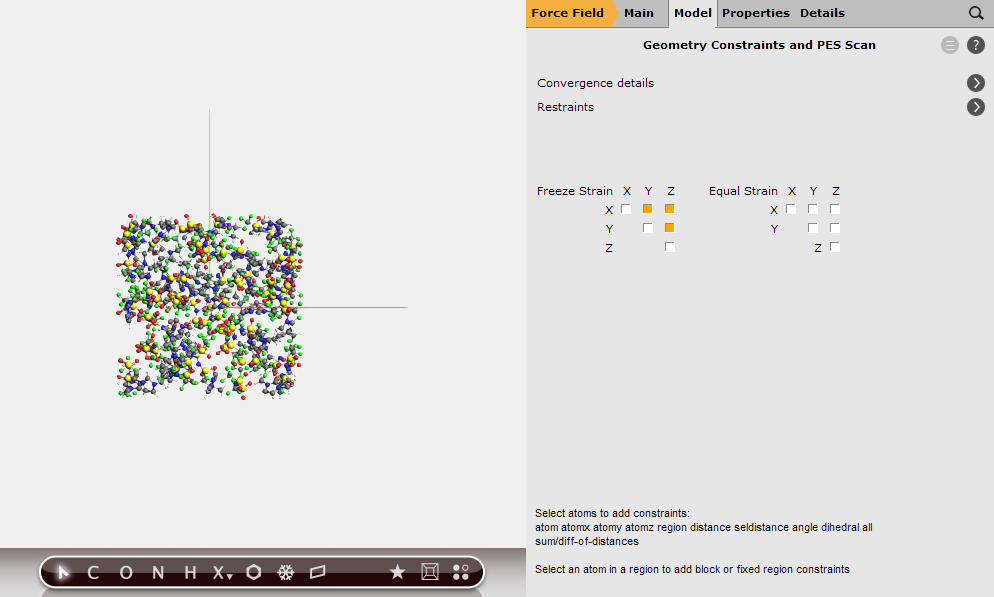
We will force the simulation box to remain orthorhombic during optimization. To this end, we will set constraints on the off-diagonal strain elements.

1. Select Task → Geometry Optimization.

2. Click on to go to the Details → Geometry Optimization panel.

3. Enable the Optimize lattice check-box.

4. Click on next to Constraints to go to the Model → Geometry constraints and PES Scan panel.

5. Enable the three off-diagonal check-boxes (XY, XZ, YZ) under Freeze Strain X Y Z

Viewing the results

This is all the setup we need. We are now ready to run the calculation. With 1360 atoms, the FIRE method may take more than a thousand steps to converge. While it is running, we can already follow its progress in AMSmovie.

1. Use the File → Run command.

2. When asked to save your input, save it with a name of your choice.

3. The AMSjobs window comes to the front and your job starts running.

4. Select your job and click SCM → Movie.

We want to check how well the bond constraints are maintained.

1. Select any two atoms connected by a bond.

2. Select Graph → Distance, Angle, Dihedral.

Note that the bond constraints are not always satisfied during a FIRE energy minimization with lattice optimization enabled. However, at the end of the optimization the constraints should be satisfied to a degree sufficient for the next calculation. If a higher degree is desired, one should tighten up the convergence criteria.

Even if the optimization did not fully converge, the final geometry should still be suitable for the subsequent step. When the optimization is finished, a Results Found dialog will pop up. Click the Yes, new job button.

Setting up molecular dynamics

Now we need to specify that we want to run a short molecular dynamics calculation and configure its details. We will start with a short MD simulation because we want to make sure that our input parameters make sense. Like the geometry optimization calculation above, the MD will also need to maintain bond constraints, which in this case is handled by the MolecularDynamics%Shake block. As with the previous calculation, we do not need to worry about this as AMSinput will add those automatically.

1. Select Task → Molecular Dynamics.

2. Click on to go to the Model → MD panel.

3. Configure 1000 steps with a time step of 1.0 fs. This will result in a 1 picosecond trajectory.

4. Set the sample frequency to 10. With a total of 1000 steps this will result in 100 recorded samples.

5. Set the Initial temperature to 393 K.

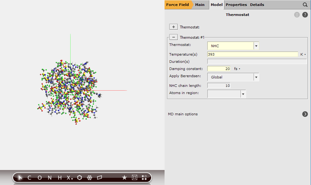
We have set an initial temperature of 393K, but in order to maintain this temperature throughout the simulation we should also attach a thermostat to our system. We will be using the Nosé–Hoover thermostat which yields good overall sampling results in general. The Nosé–Hoover damping constant is dependent on the system size because ideally it should match the period of the internal oscillations of the system. In the present case we use a reasonable value of 20 fs, but for a different system one might want to test different values.

1. Click on next to Thermostat to go to the Model → Thermostat panel.

2. Click the + button to add a thermostat to the simulation.

3. Select Thermostat → NHC (Nosé–Hoover chain).

4. Set 393 K as the Temperature.

5. Set 20 fs as the damping constant.

Since, in the end, we will probably want to reproduce the experimental density we also need to vary the volume of the simulation box. That is, we need to set up a barostat.

1. Click on next to MD main options to go back to the Model → MD panel.

2. Click on next to Barostat to go to the Model → Barostat panel.

3. Select Barostat → MTK.

4. Set 1 atm as the Pressure.

5. Set 200 fs as the damping constant.

Viewing the results

We are now ready to run the calculation. While it is running, we can already follow its progress in AMSmovie.

1. Use the File → Run command.

2. When asked to save your input, save it with a name of your choice.

3. The AMSjobs window comes to the front and your job starts running.

4. Select your job and click SCM → Movie.

Wait for the job to finish successfully, that is without error messages or warnings. If you notice that the pressure jumps wildly between large positive and negative values (say, larger than 100 MPa in magnitude) then you may need to increase the barostat damping constant. Near the end of this short simulation, the pressure should stay within the ±20 MPa (approximately ±200 bar) interval.

You are now ready to run some real MD calculations with the APPLE&P force-field. For example, you could try to reproduce the [emim][Ntf2] experimental density (1427 kg/m³, see references in O. Borodin, J. Phys. Chem. B 113, 11463–11478 (2009)) by increasing the number of MD steps in the previous example to 1 million (thus making it a 1-nanosecond equilibration) followed by another 1-nanosecond sampling run. The average density during the latter simulation should be reasonably close to the reported value. These calculations potentially take days so they go beyond the scope of the current tutorial.