Thermal conductivity via non-equilibrium molecular dynamics
In this tutorial the temperature-dependent thermal conductivity is calculated from a non-equilibrium molecular dynamics (NEMD ) trajectory. The AMS engine used is the UFF force field .
A heat flow is realized by running two local thermostats, heat source and heat sink, inside the same molecular structure. The heat source is set to be 10K above the target temperature, while the heat sink is kept 10K below the target temperature. From the energy collected at the heat sink over time and the cross-sectional area, the heat flux and thermal conductivity can be calculated. Both the molecular structure and the workflow were taken from the combined experimental and theoretical study E.M. Moscarello, B.L. Wooten, H. Sajid, L.D. Tichenor, J.P. Heremans, M.A. Addicoat, P.L. McGrier, ACS Appl. Nano Mater. 2022, 5, 10, 13787–13793.
Setup
Begin by downloading the input structure BBO_COF1.xyz. The file contains the cartesian
coordinates of a benzobisoxazole (BBO)-linked COF for which the thermal conductivity at 80K will be calculated.
Note
The periodic structure has been relaxed with GFN1-xTB (including the lattice), as described in the paper .
BBO_COF1.xyz and import them into AMSinput
Define a heat source and a heat sink by using regions .

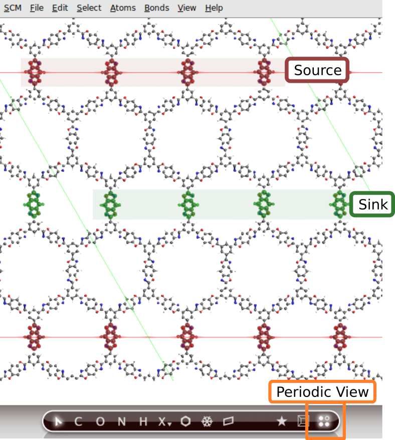
 to generate a region
source for the regionsink region
The source and sink regions can now be connected to two independent thermostats
to generate a thermostat9010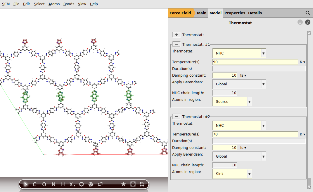
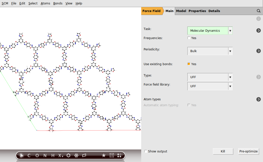
As the final step, define the settings for the molecular dynamics calculation
10000001 fs80 K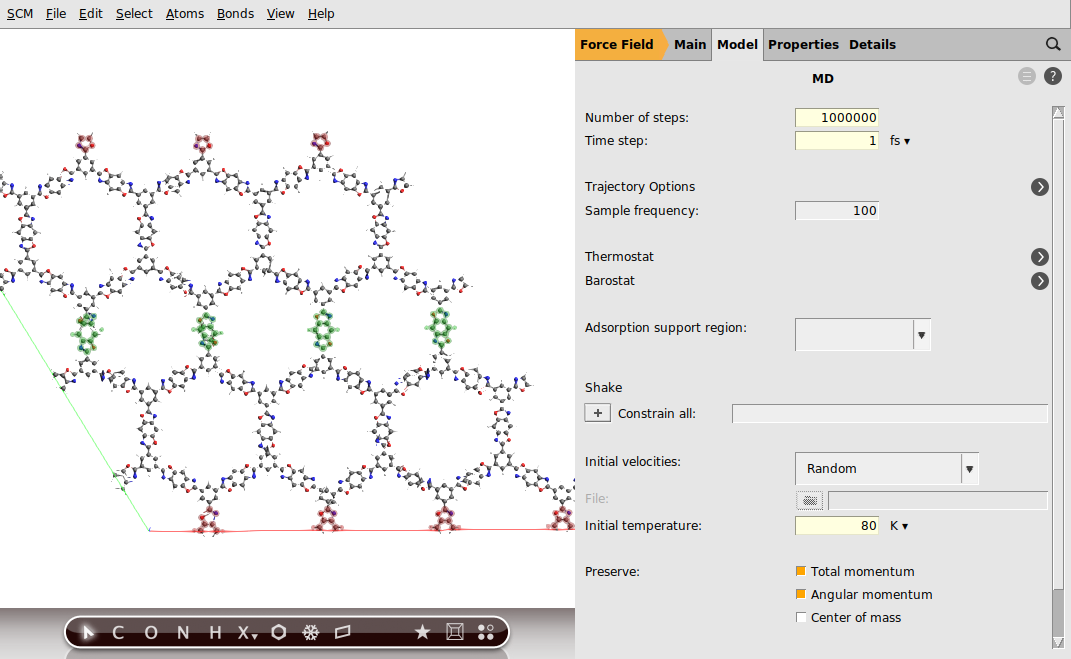
To start the calculation, do
On a recently modern 12-core desktop computer the calculation will take around 1.5 hours.
Results
Note
The calculation of the thermal conductivity requires the use of spreadsheet software such as Open Office Calc , or similar.
Once the calculation has finished we can view the results in AMSmovie.
 select AMSmovie
The relevant bits for the NEMD calculation are the energies of the two thermostats as well the time. To visualize these values:
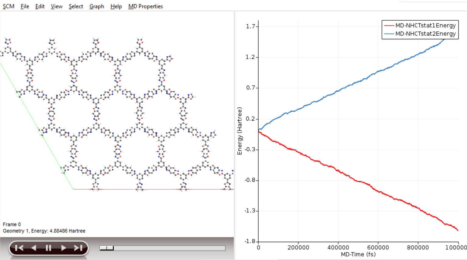
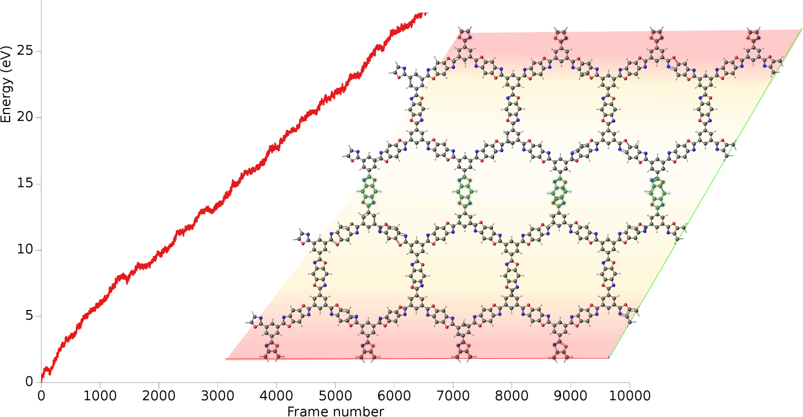
The energy of the sink thermostat is the one ascending over time, while the source is descending. To export these results into ASCII format from the GUI:
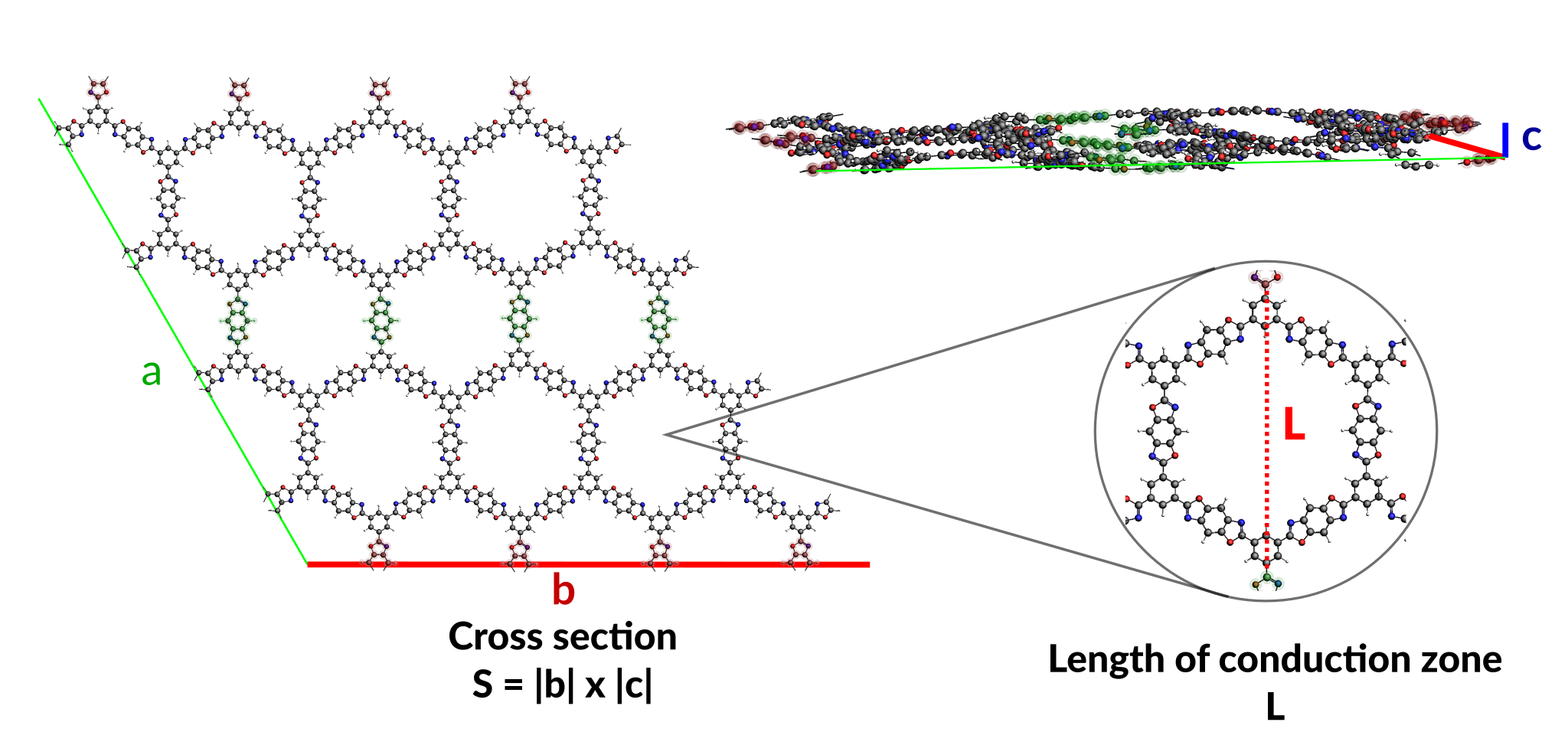
Plot the sink energy over the simulation time, as opposed to the step(!) and calculate the heat flux (Q) via
where dE/dt is the slope of the graph sink energy [Hartree, a.u.] vs. time [fs]

S is the cross-sectional area, i.e. the area from which heat enters the system, that can be calculated from the lattice vectors b and c of the system:
Tip
The lattice vectors can be found under Model → Lattice
The factor 2 stems from the periodic boundary conditions because the heat can flow in two directions. With the heat flux Q and the length of the conduction zone L, the thermal conductivity (k) can be calculated from Fourier’s law:
Note
Due to the non-deterministic nature of the MD thermostats and the fitting procedure, the result of this tutorial can vary slightly. Still, the thermal conductivity should be reasonably close to the experimental value.