2.2. Getting Started: Lennard-Jones Potential for Argon

This example illustrates how to fit a Lennard-Jones potential. The systems are snapshots from a liquid Ar MD simulation. The forces and energies (the reference data) were calculated with dispersion-corrected DFTB.

Note

In this tutorial the training data has already been prepared. See how it was generated further down.

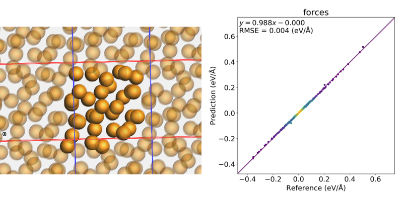
Fig. 2.1 Left: One of the systems in the job collection. Right: predicted (with parametrized Lennard-Jones) forces compared to reference (dispersion-corrected DFTB) forces.

Tip

Each step of the tutorial covers

• How to use the ParAMS graphical user interface
• How to run or view results from the command-line

2.2.1. Lennard-Jones Parameters, Engine, and Interface

The Lennard-Jones potential has the form

\[V(r) = 4\epsilon \left[\left(\frac{\sigma}{r}\right)^{12} - \left(\frac{\sigma}{r}\right)^6 \right] = \epsilon \left[\left(\frac{r_{\text{min}}}{r}\right)^{12} - 2\left(\frac{r_{\text{min}}}{r}\right)^6 \right]\]

where \(\epsilon\) and \(\sigma\) are parameters. The Lennard-Jones engine in AMS has the two parameters Eps (\(\epsilon\)) and RMin (distance at which the potential reaches a minimum), where \(\text{Rmin} = 2^{1/6}\sigma\).

In ParAMS, those two parameters can be optimized with the Lennard-Jones parameter interface, which is used in this example. The parameters then have the names eps and rmin (lowercase).

2.2.2. Files

Download LJ_Ar_example.zip and unzip the file, or make a copy of the directory $AMSHOME/scripting/scm/params/examples/LJ_Ar.

The directory contains four files (parameter_interface.yaml, job_collection.yaml, training_set.yaml, and params.conf.py) that you can view and change in the ParAMS graphical user interface (GUI). If you prefer, you can also open them in a text editor.

Start the ParAMS GUI: First open AMSjobs or AMSinput, and then select SCM → ParAMS

Select File → Open and browse to the job_collection.yaml file. This will also import the other files in the same directory.

LJ_Ar
├── job_collection.yaml
├── parameter_interface.yaml
├── params.conf.py
├── python_version.py
├── README.txt
└── training_set.yaml

The python_version.py is intended for users who prefer to write their own Python scripts rather than use the GUI and command line interface. It shows how the parameter optimization can be started using Python only and does not rely on the params.conf.py. Select the respective tabs below if this is of interest to you, otherwise the file can be ignored.

2.2.3. ParAMS input

2.2.3.1. Parameter interface (parameter_interface.yaml)

GUI

parameter_interface.yaml

Python

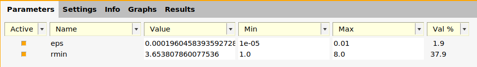
The parameters are shown on the Parameters tab.

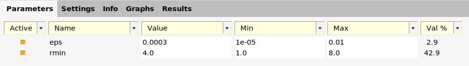
All the parameters in a parameter interface have names. For Lennard-Jones, there are only two parameters: eps and rmin.

Every parameter has a value and an allowed range of values. Above, the value for eps is shown to be 0.0003, and the allowed range to between 1e-5 and 0.01. This means that the eps variable will only be varied between \(10^{-5}\) and \(10^{-2}\) during the parametrization.

Similarly, the initial value for rmin is set to 4.0, and the allowed range is between 1.0 and 8.0.

Note

You can edit the parameter values and the allowed ranges directly in the table.

The Active attribute of the parameters is set checked, meaning that they will be optimized. To not optimize a parameter, untick the Active checkbox.

The Val % column indicates how close to the Min or Max that the current value is. It is calculated as 100*(value-min)/(max-min). For example, for rmin, it is 100*(4.0-1.0)/(8.0-1.0) = 42.9. It has no effect on the parametrization; it only lets you quickly see if the value is close to the Min or Max.

The parameter_interface.yaml file is a Parameter Interface of type LennardJonesParameters. It contains the following:

---
dtype: LennardJonesParameters
settings:
  input:
    lennardjones: {}
version: '2022.101'
---
name: eps
value: 0.0003
range:
- 1.0e-05
- 0.01
is_active: true
atoms: []
---
name: rmin
value: 4.0
range:
- 1.0
- 8.0
is_active: true
atoms: []
...

All the parameters in a parameter interface have names. For Lennard-Jones, there are only two parameters: eps and rmin.

Every parameter needs an initial value and an allowed range of values. Above, the initial value for eps is set to 0.0003, and the allowed range to between 1e-5 and 0.01. This means that the eps variable will only be varied between \(10^{-5}\) and \(10^{-2}\) during the parametrization.

Similarly, the initial value for rmin is set to 4.0, and the allowed range is between 1.0 and 8.0.

The is_active attribute of the parameters is set to True, meaning that they will be optimized.

For details about the header of the file (lines 2-6), see the parameter interface documentation.

Use the $AMSBIN/amspython program that comes with your installation of AMS. Import the params package:

from scm.params import *

Load the Lennard-Jones parameter interface:

params = LennardJonesParameters()

Note

You can iterate over parameters in an interface to view or change their values, ranges or other data:

for p in params:
    print(p.name)
    print(p.value) # initial value
    print(p.range) # optimization range
    print(p.is_active) # whether to optimize the parameter

See Parameter Interfaces for more information.

2.2.3.2. Job Collection (job_collection.yaml)

GUI

job_collection.yaml

Python

The Jobs panel contains three entries. They have the JobIDs Ar32_frame001, Ar32_frame002, and Ar32_frame003.

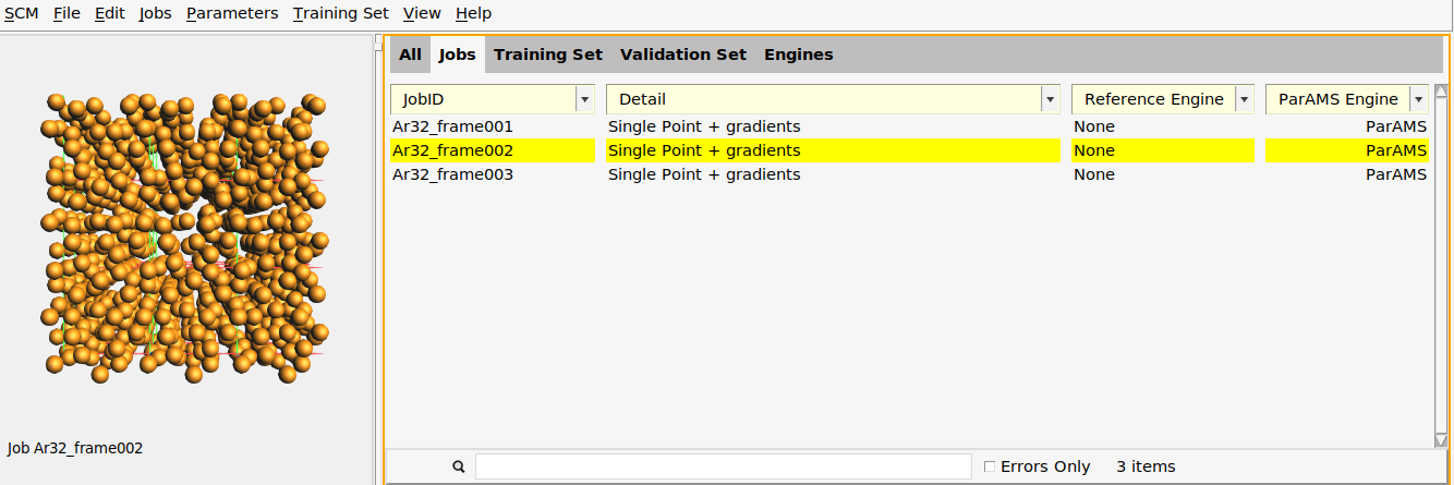
Select one of the jobs in the table.

This updates the molecule area to the left to show the structure.

You can customize how the molecule is shown just like in AMSinput, AMSmovie, etc. For example, select View → Periodic → Repeat Unit Cells to see some periodic images.

Select View → Periodic → Repeat Unit cells again to only view one periodic image.

The Jobs panel has four columns:

• JobID: The name of the job. You can rename a job directly in the table by first selecting the row, and then clicking on the job id.
• Detail: Some information about the job. SinglePoint + gradients means that a single point calculation on the structure is performed, also calculating the gradients (forces). Double-click in the Detail column for a job to see and edit the details. You can also toggle the Info panel in the bottom half.
• Reference Engine: This column can contain details about the reference calculation, and is described more in the tutorials Import training data (GUI) and Calculate reference values with ParAMS.
• ParAMS Engine: This column can contain details about job-specific engine settings. It is described in the tutorial GFN1-xTB: Lithium fluoride

The job_collection.yaml file is a Job Collection. It contains entries like these:

---
dtype: JobCollection
version: '2022.101'
---
ID: 'Ar32_frame001'
ReferenceEngineID: None
AMSInput: |
   properties
     gradients Yes
   End
   system
     Atoms
                Ar       5.1883477539      -0.4887475488       7.9660568076 
                Ar       5.7991822399       0.4024595652       2.5103286966 
                Ar       6.1338265157       5.5335946219       7.0874208384 
                Ar       4.6137188191       5.9644505949       3.0942810122 
                Ar       8.4186778390       7.6292969115       8.0729664423 
                Ar       8.3937816110       8.6402371806       2.6057806799 
                Ar       7.5320205143       1.7666481606       7.7525889818 
                Ar       8.5630139885       2.0472039529       2.6380554086 
                Ar       2.6892353632       7.8435284207       7.7883054306 
                Ar       2.4061636915       7.5716025415       2.4535180075 
                Ar       2.2485171283       2.9764130946       7.8589298904 
                Ar       3.0711058946       1.8500587164       2.5620921469 
                Ar       7.6655637500      -0.4865893003       0.0018797080 
                Ar       7.7550067215      -0.0222821825       4.8528637785 
                Ar       7.7157262425       4.6625079517      -0.3861722152 
                Ar       7.7434900996       5.2619590353       4.2602386226 
                Ar       3.4302237084      -0.2708640738       0.6280466620 
                Ar       2.8648051689       0.6106220610       6.1208342905 
                Ar       3.2529823775       5.7151788324      -0.2024448179 
                Ar       2.0046357208       4.9353027402       5.4968740217 
                Ar       0.9326855213       8.0600564695      -0.3181225099 
                Ar      -0.5654205469       8.5703446434       5.8930973456 
                Ar      -0.9561293133       2.1098403312      -0.0052667919 
                Ar      -0.8081417664       3.2747992855       5.5295389610 
                Ar       5.5571960244       7.5645919074       0.1312355350 
                Ar       4.4530832384       7.6170633330       5.4810860433 
                Ar       5.1235367625       2.7983577675      -0.3161069611 
                Ar       5.2048439076       2.9885672135       4.5193274119 
                Ar      -0.2535891591       0.0134355189       8.3061692970 
                Ar       0.5614183785      -0.1927751317       3.2355155467 
                Ar      -0.0234943080       5.0313863031       8.0451075074 
                Ar      -0.4760138873       6.2617510830       2.5759742219 
     End
     Lattice
           10.5200000000     0.0000000000     0.0000000000
            0.0000000000    10.5200000000     0.0000000000
            0.0000000000     0.0000000000    10.5200000000
     End

Each job collection entry has an ID (above Ar32_frame001) and some input to AMS, in particular the structure (atomic species, coordinates, and lattice). Each entry in the job collection constitutes a job that is run for every iteration during the parametrization.

What to extract from the jobs is defined in Training Set (training_set.yaml).

To load the Job Collection

jc = JobCollection('job_collection.yaml')

Note

The Job Collection is dict-like with key-value pairs of jobID and JCEntry, respectively. Each JCEntry stores a plams Molecule, job settings and optional metadata.

for jobid, job in jc.items():
    print(jobid)
    print(job.molecule)
    print(job.settings)
    print(job.metadata)

The Job Collection can also be used to calculate multiple jobs. See Job and Engine Collections for more information.

2.2.3.3. Training Set (training_set.yaml)

GUI

training_set.yaml

Python

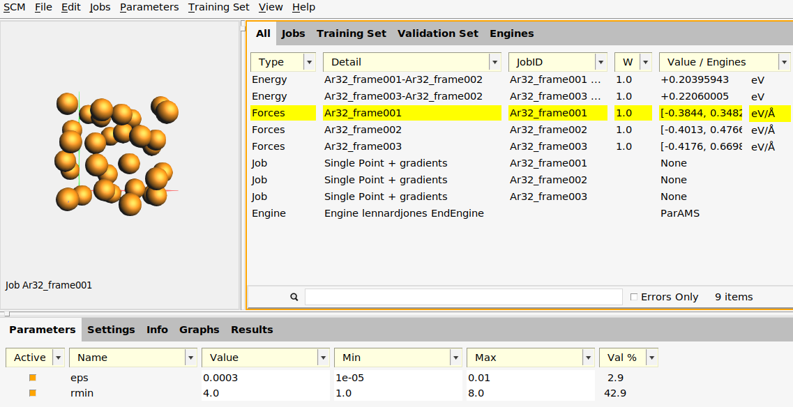
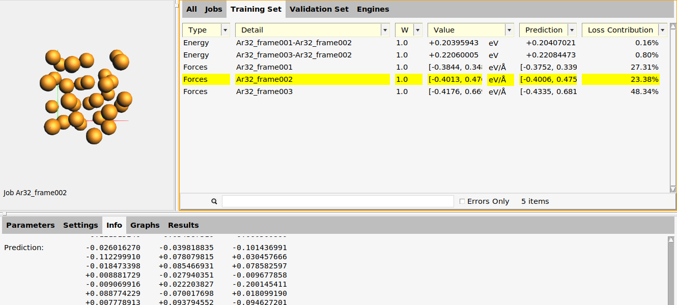
The Training Set panel contains five entries: two of type Energy and three of type Forces.

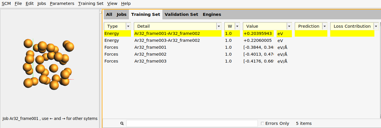
The first Energy entry has the Detail Ar32_frame001-Ar32_frame002. This means that for every iteration during the parametrization, the current Lennard-Jones parameters will be used to calculate the energy of the job Ar32_frame001 minus the energy of the job Ar32_frame002. The number should ideally be as close as possible to the reference value, which is given as 0.204 eV in the Value column. The greater the deviation from the reference value, the more this entry will contribute to the loss function.

Double-click in the Detail column for the first entry to see some more details.

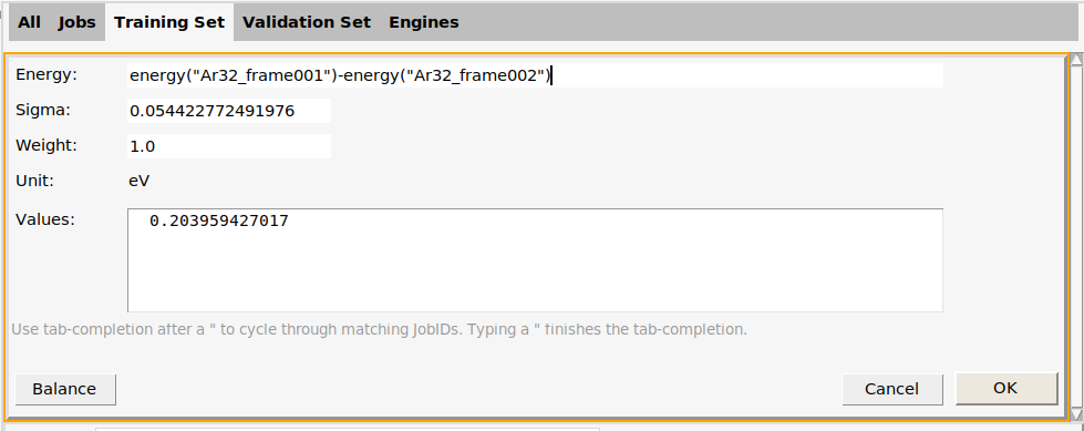
This brings up a dialog where you can change

• What is calculated (the Energy text box). For example, energy("Ar32_frame001") extracts the energy of the Ar32_frame001 job. You can combine an arbitrary number of such energies with normal arithmetic operations (+, -, /, *). For details, see the Import training data (GUI) tutorial.
• Sigma: A number signifying an “acceptable prediction error”. Here, it is given as 0.0544 eV, which is the default value for energies. A smaller sigma will make the training set entry more important (contribute more to the loss function). For beginning ParAMS users, we do not recommend to modify Sigma, but instead to modify the Weight.
• Weight: A number signifying how important the training set entry is. A larger weight will make the training set entry more important (contribute more to the loss function). The default weight is 1.0.

Note

The Sigma for a training set entry is not the σ that appears in the Lennard-Jones equation. For more information about Sigma and Weight, see Sigma vs. weight: What is the difference?.

• Unit: The unit that Sigma and the reference value are expressed in. Here, it is set to eV. See how to set preferred units.
• Value: The reference value (expressed in the unit above).

Click OK. This brings you back to the Training Set panel.

The W column contains the Weight of the training set entry. You can edit it directly in the table.

The Value column contains the reference value.

The Prediction column contains the predicted value (for the “best” parameter set) for running or finished parametrizations. It is now empty.

The Loss contribution column contains the how much an entry contributes to the loss function (in percent) for running or finished parametrizations. It is now empty.

Many different quantities can be extracted from a job. The third entry is of type Forces for the job Ar32_frame001. The reference data are the atomic forces (32 × 3 force components) from the job Ar32_frame001. The Value column gives a summary: [-0.3844, 0.3482] (32×3), meaning that the most negative force component is -0.3844 eV/Å, and the most positive force component is +0.3482 eV/Å.

To see all force components, either double-click in the Details column or switch to the Info panel at the bottom.

The training_set.yaml file is a Data Set. It contains entries like these:

---
dtype: DataSet
version: '2022.101'
---
Expression: energy('Ar32_frame001')-energy('Ar32_frame002')
Weight: 1.0
Sigma: 0.054422772491975996
ReferenceValue: 0.20395942701637979
Unit: eV, 27.211386245988
---
Expression: energy('Ar32_frame003')-energy('Ar32_frame002')
Weight: 1.0
Sigma: 0.054422772491975996
ReferenceValue: 0.22060005303998803
Unit: eV, 27.211386245988
---
Expression: forces('Ar32_frame001')
Weight: 1.0
Sigma: 0.15426620242897765
ReferenceValue: |
   array([[ 0.04268692, -0.02783233,  0.04128417],
          [ 0.02713834, -0.04221017, -0.01054571],
          [-0.00459236, -0.07684888,  0.06155902],
          [ 0.34815492, -0.38436427, -0.12292068],
          [-0.20951048, -0.09704763,  0.30684271],
          [-0.12165704,  0.02841069, -0.03455513],
          [-0.01065992,  0.04707562, -0.00797079],
          [-0.09806036,  0.06893426,  0.29291125],
          [-0.08117544,  0.00197622,  0.05092921],
          [-0.26343319,  0.26285542, -0.02473382],
          [ 0.06144345, -0.01781664,  0.17121465],
          [-0.16915463,  0.24386843,  0.13151148],
          [-0.01651514,  0.03927323, -0.12482729],
          [-0.05972447,  0.09258089,  0.23253252],
          [ 0.00554623,  0.0802643 ,  0.00565681],
          [-0.14037904,  0.02969844,  0.01099823],
          [-0.03492464, -0.20821058, -0.25464835],
          [-0.01710259, -0.10689741, -0.13469458],
          [-0.12217555, -0.15624485, -0.02885505],
          [ 0.04492738,  0.08596881, -0.11475184],
          [-0.15375715,  0.02301999,  0.09411744],
          [ 0.26855338,  0.0068943 , -0.31912743],
          [ 0.19519975,  0.05424052, -0.29197409],
          [ 0.03589698, -0.11822402,  0.00851084],
          [ 0.12697447,  0.08277883,  0.01592771],
          [ 0.10473145,  0.18847622, -0.03627933],
          [-0.03520977, -0.03814586,  0.0023055 ],
          [ 0.05408552,  0.02290898,  0.08376102],
          [ 0.06093887,  0.00964534, -0.01148707],
          [ 0.02291482,  0.01746282,  0.00389746],
          [-0.07331299,  0.09730838,  0.08506009],
          [ 0.21215231, -0.20979905, -0.08164896]])
Unit: eV/angstrom, 51.422067476325886
---

The first entry has the Expression

Expression: energy('Ar32_frame001')-energy('Ar32_frame002')

which means that for every iteration during the parametrization, the current Lennard-Jones parameters will be used to calculate the energy of the job Ar32_frame001 minus the energy of the job Ar32_frame002. The number should ideally be as close as possible to the ReferenceValue, which above is given as 0.204 eV. The greater the deviation from the reference value, the more this entry will contribute to the loss function.

The Weight and Sigma also affect how much the entry contributes to the loss function. For details, see Data Set and Sigma vs. weight: What is the difference?.

Note

The Sigma in training_set.yaml is not the \(\sigma\) that appears in the Lennard-Jones equation.

Reference data can be expressed in any Unit. The Unit for the first expression is given as eV, 27.21138. The number specifies a conversion factor from the default unit Ha. If no Unit is given, the data must be given in the default unit.

Many different quantities can be extracted from a job. The third entry (starting on line 17) has the Expression

Expression: forces('Ar32_frame001')

which extracts the atomic forces (32 × 3 force components) from the job Ar32_frame001. The reference value for the force components are given as a matrix in eV/angstrom (as specified by the Unit).

A training set is loaded with

ts = DataSet('training_set.yaml')

Note

The Data Set defines which properties need to be extracted and compared from the jobs in a Job Collection. This is defined through an expression string. Weights can be used to tune the relative importance of a property. It also stores the reference value – used during fitting – for each entry.

for entry in ts:
    print(entry.expression)
    print(entry.weight)
    print(entry.reference)

2.2.3.4. ParAMS settings (params.conf.py)

GUI

params.conf.py

Python

Open the Settings panel in the bottom half.

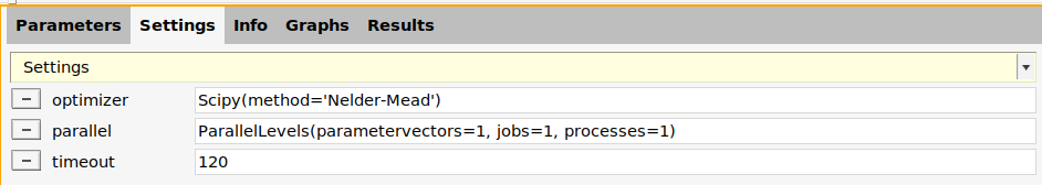
There are three lines:

• optimizer: Scipy(method='Nelder-Mead')
• parallel: ParallelLevels(parametervectors=1, jobs=1, processes=1)
• timeout: 120

Optimizer: The optimizer variable is an Optimizer. For simple optimization problems like Lennard-Jones, the Nelder-Mead method from scipy can be used. For more complicated problems, like ReaxFF optimization, a more advanced optimizer like the CMAOptimizer is recommended (see for example the ReaxFF: Gaseous H₂O tutorial).

Parallellization: The parallel variable is a ParallelLevels, specifying how to parallelize the parameter optimization. Here, it is explicitly set to run in serial. If you remove the option by clicking the button, that will instead try to use an optimal parallelization strategy for your machine.

Timeout: The timeout variable gives the maximum number of seconds that the parametrization is allowed to run. If the parametrization takes longer than two minutes (120 seconds), it will stop. If you remove the option by clicking the button, then there is no time limit.

There are also a few more options. Click the yellow Settings drop-down to add other options. Their meaning can be found in the ParAMS Main Script documentation.

The params.conf.py file contains

### The training_set, job_collection, and parameter_interface variables contain paths to the corresponding .yaml files
training_set = 'training_set.yaml'   
job_collection = 'job_collection.yaml'
parameter_interface = 'parameter_interface.yaml'

### Define an optimizer for the optimization task. Use either a CMAOptimizer or Scipy
#optimizer = CMAOptimizer(sigma=0.1, popsize=10, minsigma=5e-4) 
optimizer = Scipy(method='Nelder-Mead')

### run the optimization in serial
parallel = ParallelLevels(parametervectors=1, jobs=1, processes=1)

### Stop the optimization after 2 minutes if it has not finished with the timeout variable.
timeout = 120

Variables: The training_set, job_collection, parameter_interface, optimizer, parallel, and timeout variables are interpreted by when running the optimization.

Optimizer: The optimizer variable is an Optimizer. For simple optimization problems like Lennard-Jones, the Nelder-Mead method from scipy can be used. For more complicated problems, like ReaxFF optimization, a more advanced optimizer like the CMAOptimizer is recommended.

Parallellization: The parallel variable is a ParallelLevels, specifying how to parallelize the parameter optimization. Set it to None to use a good default for your machine.

Timeout: The timeout variable gives the maximum number of seconds that the parametrization is allowed to run. If the parametrization takes longer than two minutes (120 seconds), it will stop. If not given, then there is no time limit.

There are also a few more options. See the ParAMS Main Script documentation.

Any available optimizer can be selected for a parameter optimization:

optimizer = Scipy('Nelder-Mead')

We recommend using CMA-ES for initial production.

Parallelization is controlled by the ParallelLevels class:

parallel = ParallelLevels(parametervectors=1, jobs=1)

By default, parallelization will default to evaluating as many parameter vectors as possible in parallel. In most cases this will be optimal for ReaxFF optimizations (where the time ratio of AMS startup to single job evaluation is high).

Callbacks control various interactions with a running Optimization. They are meant to provide additional statistics or determine when an optimization should stop:

callbacks = [Timeout(60*2)] # 2 min

2.2.4. Run the example

GUI

Command-line

Python

Save the project with a new name. If the name does not end with .params, then .params will be added to the name.

File → Save As with the name lennardjones.params

File → Run

This brings up an AMSjobs window.

Go back to the ParAMS window.

While the parameterization is running, go to the Graphs panel at the bottom.

There, you can see some graphs automatically updating. These show you the current “best” results in a variety of different ways. They will be explained in more detail later.

Tip

Using AMSjobs you can also submit ParAMS jobs to remote queues (compute clusters).

Start a terminal window as follows:

• Windows: In AMSjobs, select Help → Command-line, type bash and hit Enter.
• MacOS: In AMSjobs, select Help → Terminal.
• Linux : Open a terminal and source /path/to/ams/amsbashrc.sh

In the terminal, go to the LJ_Ar directory, and run the ParAMS Main Script:

"$AMSBIN/params" optimize

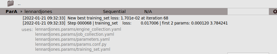
which gives beginning output similar to this:

[2021-12-06 10:07:21]  Reading ParAMS config ...
[2021-12-06 10:07:21]    Loading job collection from job_collection.yaml ... [2021-12-06 10:07:21]  done.
[2021-12-06 10:07:21]    Loading data training set from training_set.yaml ... [2021-12-06 10:07:21]  done.
[2021-12-06 10:07:21]  Checking project for consistency ...
[2021-12-06 10:07:21]  No issues found.
[2021-12-06 10:07:21]  Starting parameter optimization. Dim = 2
[2021-12-06 10:07:21]  Initial loss: 5.722e+02
[2021-12-06 10:07:21]  New best training_set loss: 5.722e+02 at iteration 0
[2021-12-06 10:07:21]  Step 000000 | training_set    loss:      572.188673 | first 2 params: 0.000300 4.000000
[2021-12-06 10:07:21]  New best training_set loss: 5.722e+02 at iteration 1
[2021-12-06 10:07:21]  Step 000001 | training_set    loss:      572.188673 | first 2 params: 0.000300 4.000000
[2021-12-06 10:07:21]  New best training_set loss: 5.062e-01 at iteration 2
[2021-12-06 10:07:21]  Step 000002 | training_set    loss:        0.506209 | first 2 params: 6.47500000e-05 4.000000
[2021-12-06 10:07:22]  New best training_set loss: 7.795e-02 at iteration 4
[2021-12-06 10:07:22]  Step 000004 | training_set    loss:        0.077947 | first 2 params: 6.47500000e-05 3.975000
[2021-12-06 10:07:22]  Step 000010 | training_set    loss:             inf | first 2 params: 5.93750000e-06 3.990625
[2021-12-06 10:07:22]  New best training_set loss: 6.769e-02 at iteration 19
[2021-12-06 10:07:22]  Step 000019 | training_set    loss:        0.067688 | first 2 params: 6.19931641e-05 3.986084
[2021-12-06 10:07:22]  Step 000020 | training_set    loss:        0.351541 | first 2 params: 6.93447266e-05 3.973193
[2021-12-06 10:07:22]  New best training_set loss: 5.458e-02 at iteration 21
[2021-12-06 10:07:22]  Step 000021 | training_set    loss:        0.054580 | first 2 params: 6.03850098e-05 3.984216
[2021-12-06 10:07:23]  New best training_set loss: 5.222e-02 at iteration 24
[2021-12-06 10:07:23]  Step 000024 | training_set    loss:        0.052219 | first 2 params: 6.04998779e-05 3.987921
[2021-12-06 10:07:23]  New best training_set loss: 5.095e-02 at iteration 27
[2021-12-06 10:07:23]  Step 000027 | training_set    loss:        0.050946 | first 2 params: 6.11316528e-05 3.983298
[2021-12-06 10:07:23]  New best training_set loss: 4.973e-02 at iteration 30
[2021-12-06 10:07:23]  Step 000030 | training_set    loss:        0.049733 | first 2 params: 6.26680145e-05 3.976600
[2021-12-06 10:07:23]  New best training_set loss: 4.857e-02 at iteration 31
[2021-12-06 10:07:23]  Step 000031 | training_set    loss:        0.048568 | first 2 params: 6.37520828e-05 3.970939
[2021-12-06 10:07:23]  New best training_set loss: 4.832e-02 at iteration 33

The starting parameters were eps=0.0003 and rmin=4.0 (as can be seen on the line starting with Step 000000). Every 10 iterations, or whenever the loss function decreases, the current value of the loss function is printed. The goal of the parametrization is to minimize the loss function. It should take less than a minute for the parametrization to finish.

The Optimization class brings all the above together into one task:

O = Optimization(
    job_collection=jc,
    data_sets=ts,
    parameter_interface=params,
    optimizer=optimizer,
    callbacks=callbacks,
    parallel=parallel,
    workdir='optimization',
)

It can be started with the optimize() method

O.optimize()

2.2.5. Parametrization results

2.2.5.1. The best parameter values

GUI

Command-line

The best (optimized) parameters are shown on the Parameters tab in the bottom half of the window. They get automatically updated as the optimization progresses.

You can also find them in the file lennardjones.results/optimization/training_set_results/best/lj_parameters.txt (or lennardjones.results/optimization/training_set_results/best/parameter_interface.yaml):

Engine LennardJones
    Eps 0.00019604583935927278
    RMin 3.653807860077536
EndEngine

Tip

To use the optimized parameters in a new simulation, open AMSinput and switch to the Lennard-Jones panel. Enter the values of the parameters and any other simulation details.

The best (optimized) parameters can be found in the file optimization/training_set_results/best/lj_parameters.txt (or optimization/training_set_results/best/parameter_interface.yaml):

Engine LennardJones
    Eps 0.00019604583935927278
    RMin 3.653807860077536
EndEngine

2.2.5.2. Correlation plots

GUI

Command-line

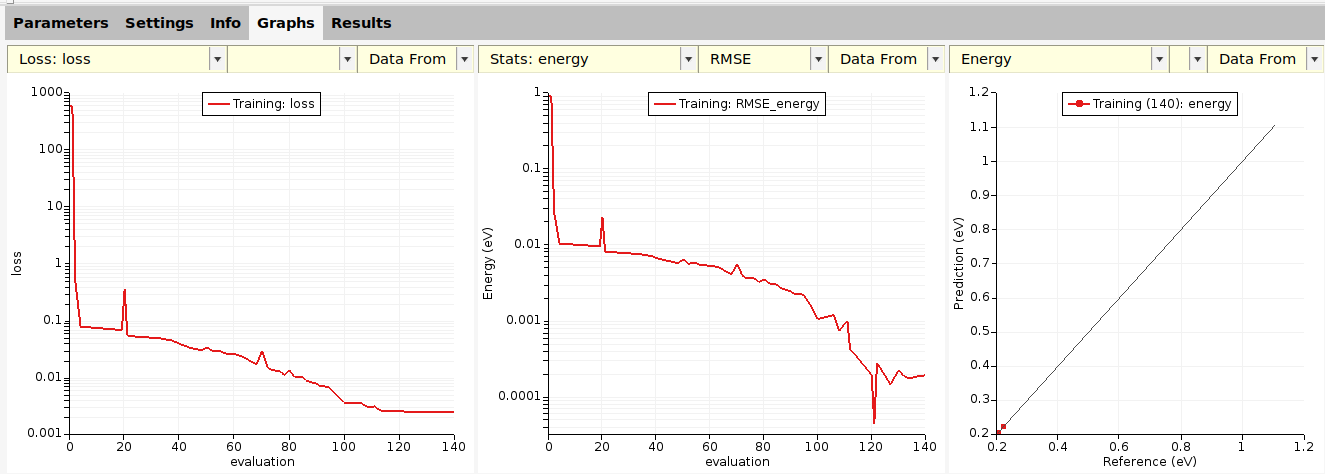
Go to the Graphs panel. There are three curves shown:

• The loss function vs. evaluation number
• The RMSE (root mean squared error) of energy predictions vs. evaluation number
• A scatter plot of predicted vs. reference energies

There are many different types of graphs that you can plot. To plot a correlation plot between the predicted and reference forces:

In the drop-down that currently says Energy, choose Forces

Click on one of the plotted points

This selects the corresponding Job in the table above

In the 3D area the atom for the force component you clicked is selected

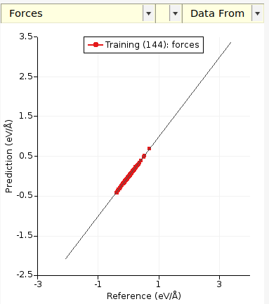
The black diagonal line is the line y = x. In this case, the predicted forces are very close to the reference forces! Let’s compare to the initially predicted forces, i.e. let’s compare the optimized parameters eps = 0.000196 and rmin = 3.6538 (from evaluation 144) to the initial parameters eps = 0.0003 and rmin = 4.0 (from evaluation 0):

In the Data From dropdown above the correlation plot, tick Training(initial): forces.

This adds a set of green datapoints with the initial predictions.

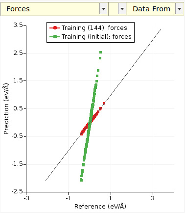
There is a third drop-down where you can choose whether to plot the Best or Latest training data. In this example, both correspond to evaluation 144. In general, the latest evaluation doesn’t have to be the best. This is especially true for other optimizers like the CMA optimizer (recommended for ReaxFF).

Go to the directory optimization/training_set_results/best/scatter_plots, and run

"$AMSBIN"/params plot forces.txt

This creates a plot similar to the one shown in the beginning of this tutorial.

2.2.5.3. Error plots

GUI

Command-line (running_loss.txt, running_stats.txt)

Go to the Graphs panel.

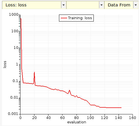
The left-most plot shows the evolution of the loss function with evaluation number. The goal of the parametrization is to minimize the loss function.

By default, the loss function value is saved every 10 evaluations or whenever it decreases.

You can also choose between the RMSE and MAE (mean absolute error) for energies and forces (and other predicted properties):

In the drop-down that says Stats: Energy, choose Stats → Forces

This plots the RMSE of the forces vs. evaluation number

In the drop-down that says RMSE, choose MAE

This plots the MAE of the forces vs. evaluation number

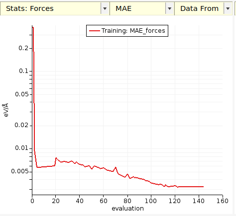
By default, the RMSE and MAE are saved every 10 evaluations or whenever the loss function decreases.

In the optimization/training_set_results/ directory are two files running_loss.txt and running_stats.txt.

These files can easily be imported into a spreadsheet (Excel) for plotting, or plotted with, for example, gnuplot.

For running_loss.txt, you can also use ParAMS’s builtin plotting tool:

"$AMSBIN"/params plot running_loss.txt

Fig. 2.2 Loss function (logscale) vs. iteration number. After about 100 iterations, the loss function value converges.

2.2.5.4. Parameter plots

GUI

Command-line (running_active_parameters.txt)

In the bottom table, switch to the Graphs panel.

In one of the drop-downs, choose Active Parameters: eps.

This plots the value of the eps parameter vs. evaluation number

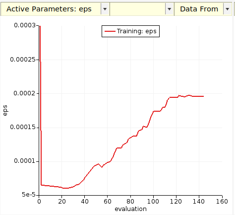
The parameters are by default saved every 500 evaluations, or whenever the loss function decreases.

You can similarly plot the rmin parameter.

Mouse-over the graph to see the value of the parameter at that iteration.

The best parameter values are shown on the Parameters tab.

The file optimization/training_set_results/best/running_active_parameters.txt contains the parameter values vs. evaluation number.

As before, this can be plotted using ParAMS:

"$AMSBIN"/params plot running_active_parameters.txt

2.2.5.5. Editing and Saving Plots

All of the above GUI plots can be customized to your liking by double clicking anywhere on one of the plot axes. This brings up a window allowing you to configure various graph options like scales, labels, limits, titles, etc.

To save the plot:

File → Save Graph As Image

Select one of the three plots to save

Choose file name and Save

If you would like to extract the raw data from the plot in .xy format:

File → Export Graph As XY

Select one of the three plots to save

Choose file name and Save

2.2.5.6. Predicted values

GUI

Command-line (data_set_predictions.yaml, energy.txt, forces.txt)

Switch to the Training Set panel in the upper table.

The Prediction column contains the predicted values (for the best evaluation, i.e., the one with the lowest loss function value). For the forces, only a summary of the minimum and maximum value is given. To see all predicted, values select one of the Forces entries and go to the Info panel at the bottom and scroll down.

You can also view the predicted values in a different way:

Switch to the Results panel in the bottom table

In the drop-down, select Training best: energy

This shows the file lennardjones.results/optimization/training_set_results/best/scatter_plots/energy.txt

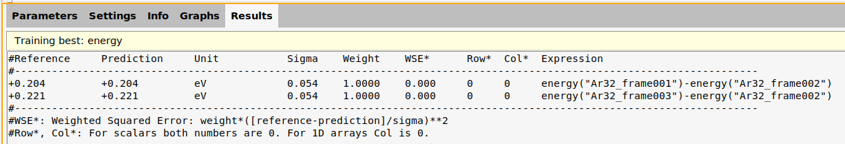
This shows a good agreement between the predicted and reference values for the relative energies in the training set.

In the drop-down, select Training best: forces

This shows the file lennardjones.results/optimization/training_set_results/best/scatter_plots/forces.txt

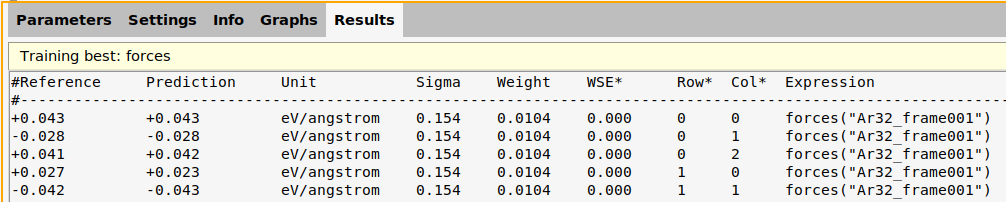
energy.txt and forces.txt are the files that are plotted when making Correlation plots.

There is one file for every extractor in the training set.

The predicted values can be viewed in:

• optimization/training_set_results/best/data_set_predictions.yaml. This file has the same format as training_set.yaml, but contains also the predicted values.
• optimization/training_set_results/best/scatter_plots/energy.txt (or forces.txt).

For example, the latter file contains

#Reference     Prediction     Unit           Sigma    Weight    WSE*      Row*  Col*  Expression
#------------------------------------------------------------------------------------------------------------------------
+0.204         +0.204         eV             0.054    1.0000    0.000     0     0     energy('Ar32_frame001')-energy('Ar32_frame002')
+0.221         +0.221         eV             0.054    1.0000    0.000     0     0     energy('Ar32_frame003')-energy('Ar32_frame002')
#------------------------------------------------------------------------------------------------------------------------
#WSE*: Weighted Squared Error: weight*([reference-prediction]/sigma)**2
#Row*, Col*: For scalars both numbers are 0. For 1D arrays Col is 0.

This shows a good agreement between the predicted and reference values for the relative energies in the training set.

2.2.5.7. Loss contributions

GUI

Command-line (data_set_predictions.yaml, stats.txt)

In the top table, switch to the Training Set panel.

The last column contains the Loss Contribution. For each training set entry, it gives the fraction that the entry contributes to the loss function value.

Here, for example, the two Energy entries only contribute 0.96% to the loss function, and the three Forces entries contribute 99.04%. If you notice that some entries have a large contribution to the loss function, and that this prevents the optimization from progressing, you may consider decreasing the weight of those entries.

The loss contribution is printed in the files

• optimization/training_set_results/best/data_set_predictions.yaml
• optimization/training_set_results/best/stats.txt

2.2.5.8. Summary statistics

GUI

Command-line (stats.txt)

In the bottom table, switch to the Results panel.

In the drop-down, select Training best: stats

This shows the file lennardjones.results/optimization/training_set_results/best/stats.txt

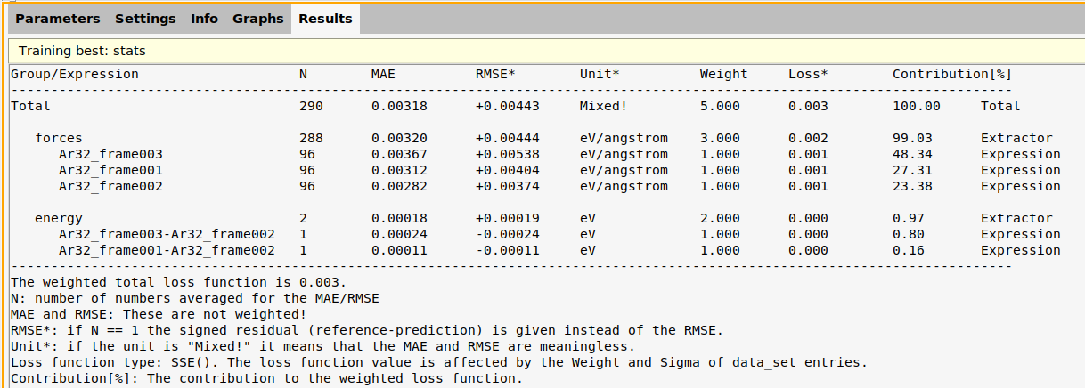
Open the file optimization/training_set_results/best/stats.txt

Group/Expression                    N        MAE          RMSE*        Unit*          Weight     Loss*        Contribution[%]
-----------------------------------------------------------------------------------------------------------------------------
Total                               290      0.00318      +0.00443     Mixed!         5.000      0.003        100.00     Total

   forces                           288      0.00320      +0.00444     eV/angstrom    3.000      0.002        99.03      Extractor
      Ar32_frame003                 96       0.00367      +0.00538     eV/angstrom    1.000      0.001        48.34      Expression
      Ar32_frame001                 96       0.00312      +0.00404     eV/angstrom    1.000      0.001        27.31      Expression
      Ar32_frame002                 96       0.00282      +0.00374     eV/angstrom    1.000      0.001        23.38      Expression

   energy                           2        0.00018      +0.00019     eV             2.000      0.000        0.97       Extractor
      Ar32_frame003-Ar32_frame002   1        0.00024      -0.00024     eV             1.000      0.000        0.80       Expression
      Ar32_frame001-Ar32_frame002   1        0.00011      -0.00011     eV             1.000      0.000        0.16       Expression
-----------------------------------------------------------------------------------------------------------------------------
The weighted total loss function is 0.003.
N: number of numbers averaged for the MAE/RMSE
MAE and RMSE: These are not weighted!
RMSE*: if N == 1 the signed residual (reference-prediction) is given instead of the RMSE.
Unit*: if the unit is "Mixed!" it means that the MAE and RMSE are meaningless.
Loss function type: SSE(). The loss function value is affected by the Weight and Sigma of data_set entries.
Contribution[%]: The contribution to the weighted loss function.

This file gives the mean absolute error (MAE) and root-mean-squared error (RMSE) per entry in the training set. The column N gives how many numbers were averaged to calculate the MAE or RMSE.

For example, in the row forces the N is 288 (the total number of force components in the training set), and the MAE taken over all force components is 0.00320 eV/Å. In the row Ar32_frame003, the N is 96 (the number of force components for job Ar32_frame003), and the MAE is 0.00367 eV/Å.

Further down in the file are the energies. In the row energy the N is 2 (the total number of energy entries in the training set). The entry Ar32_frame003-Ar32_frame002 has N = 1, since the energy is just a single number. In that case, the MAE and RMSE would be identical, so the file gives the absolute error in the MAE column and the signed error (reference - prediction) in the RMSE column.

The file also gives the weights, loss function values, and loss contributions of the training set entries. The total loss function value is printed below the table.

2.2.5.9. All output files

The GUI stores all results in the directory jobname.results (here lennardjones.results).

The results from the optimization are stored in the optimization directory:

.
└── optimization
    ├── settings_and_initial_data
    │   └── data_sets
    ├── summary.txt
    └── training_set_results
        ├── best
        │   ├── pes_predictions
        │   └── scatter_plots
        ├── history
        │   ├── 000000
        │   │   ├── pes_predictions
        │   │   └── scatter_plots
        │   └── 000144
        │       ├── pes_predictions
        │       └── scatter_plots
        ├── initial
        │   ├── pes_predictions
        │   └── scatter_plots
        └── latest
            ├── pes_predictions
            └── scatter_plots

• The settings_and_initial_data directory contains compressed versions of the job collection, training set, and parameter interface.
• The training_set_results directory contains detailed results for the training set.

The training_set_results directory contains the following subdirectories:

• The best subdirectory contains detailed results for the iteration with the lowest loss function value
• The history subdirectory contains detailed results that are stored regularly during the optimization (by default every 500 iterations).
• The initial subdirectory contains detailed results for the first iteration (with the initial parameters).
• The latest subdirectory contains detailed results for the latest iteration.

In this tutorial, both the best and latest evaluations were evaluation 144. In general, the latest evaluation doesn’t have to be the best. This is especially true for other optimizers like the CMA optimizer (recommended for ReaxFF).

• running_loss.txt : Loss function vs. evaluation
• running_active_parameters.txt : Parameters vs. evaluation
• running_stats.txt : MAE and RMSE per extractor vs. evaluation
• best/active_parameters.txt : List of the parameter values
• best/data_set_predictions.yaml : File storing the training set with both the reference values and predicted values. The file can be loaded in Python (with a Data Set Evaluator) to regenerate (modified version of) stats.txt, scatter_plots/energy.txt, etc.
• best/engine.txt : an AMS Engine settings input block for the parameterized engine.
• best/evaluation.txt : the evaluation number
• best/lj_parameters.txt : The parameters in a format that can be read by AMS. Here, it is identical to engine.txt. For ReaxFF parameters, you instead get a file ffield.ff. For GFN1-xTB parameters, you get a folder called xtb_files.
• best/loss.txt : The loss function value
• best/parameter_interface.yaml : The parameters in a format that can be read by ParAMS
• best/pes_predictions/ : A directory containing results for PES scans: bond scans, angle scans, and volume scans. It is empty in this tutorial. For an example, see ReaxFF: Gaseous H₂O.
• best/scatter_plots/ : Directory containing energy.txt, forces.txt, etc. Each file contains a table of reference and predicted values for creating scatter/correlation plots.
• best/stats.txt : Contains MAE/RMSE/Loss contribution for each training set entry sorted in order of decreasing loss contribution.

2.2.5.10. summary.txt

The optimization/summary.txt file contains a summary of the job collection, training set, and settings:

Optimization() Instance Settings:
=================================
Workdir:                           LJ_Ar/optimization/optimization
JobCollection size:                3
Interface:                         LennardJonesParameters
Active parameters:                 2
Optimizer:                         Scipy
Parallelism:                       ParallelLevels(optimizations=1, parametervectors=1, jobs=1, processes=1, threads=1)
Verbose:                           True
Callbacks:                         Logger
                                   Timeout
                                   Stopfile
PLAMS workdir path:                /tmp

Evaluators:
-----------
Name:                              training_set (_LossEvaluator)
Loss:                              SSE
Evaluation frequency:              1

Data Set entries:                  5
Data Set jobs:                     3
Batch size:                        None

Use PIPE:                          True
---
===
Start time: 2021-12-06 10:07:21.681185
End time:   2021-12-06 10:07:32.125530

2.2.6. Close the ParAMS GUI

When you close the ParAMS GUI (File → Close), you will be asked whether to save your changes.

This question might appear strange since you didn’t make any changes after running the job.

The reason is that ParAMS auto-updates the table of parameters while the parametrization is running, and also automatically reads the optimized parameters when you open the project again. To revert to the initial parameters, choose File → Revert Parameters.

If you save the changes, this will save the optimized parameters as the “new” starting parameters, which could be used as a starting point for further parametrization.

We do not recommend to overwrite the same folder several times with different starting parameters. Instead, if you want to save after having made changes to the parameters, use File → Save As and save in a new directory.

2.2.7. Appendix: Creation of the input files

GUI

Python

How to run the reference calculations and import the results into ParAMS is explained in the Import training data (GUI) tutorial. The data for this Lennard-Jones tutorial was generated following the section MD with fast method followed by Replay with reference method.

The params.conf.py file is a modified version of the standard params.conf.py file that can be generated with this command:

$AMSBIN/params makeconf

The parameter_interface.yaml, job_collection.yaml, training_set.yaml files were created with a script combining functionality from PLAMS and ParAMS. Download the script if you would like to try it. It sets up a molecular dynamics simulation of liquid Ar with the UFF force field. Some snapshots are recalculated with dispersion-corrected DFTB (GFN1-xTB). A ResultsImporter then extracts the forces and relative energies, and creates the job_collection.yaml and training_set.yaml files.

See also

Import training data (Python)

2.2.8. Next steps

• Try the ReaxFF: Gaseous H₂O or GFN1-xTB: Lithium fluoride tutorial.
• Learn how to import your own training data into ParAMS. If you already have a ReaxFF training set for use with AMS up to version 2021, it can be directly converted to ParAMS format
• Learn more about training and validation sets.
• For detailed Python tutorials see ReaxFF: Gaseous H₂O or The params Python library, or check out the documentation.