2.5. ReaxFF: Gaseous H₂O

This example shows how to fit a ReaxFF force field to reproduce a DFT-calculated H–OH bond dissociation curve of a water molecule in the gas phase.

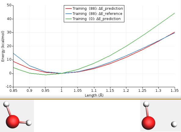
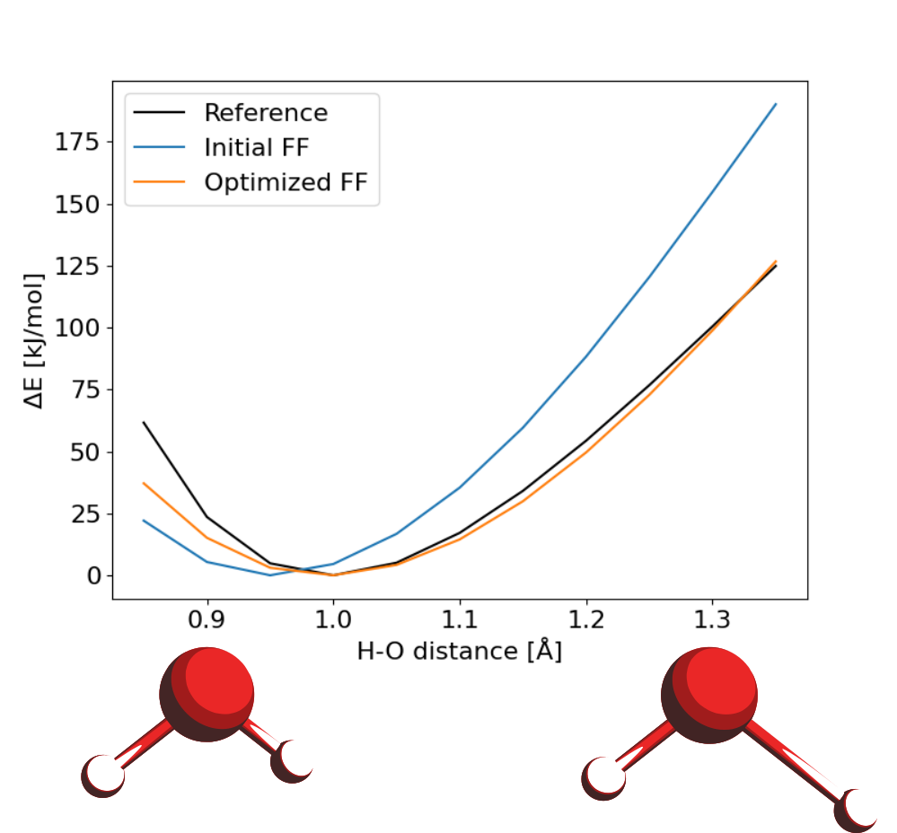
Fig. 2.3 Bond length scan of a water molecule using Water2017.ff (initial, green), DFT (reference, blue), and refitted ReaxFF force field in this tutorial (red). The (88) means that the best fit was obtained for evaluation 88.

The ReaxFF force field Water2017.ff (DOI: 10.1021/acs.jpcb/7b02548) is used as a starting point for the parametrization.

Note

The Water2017.ff force field was originally optimized for liquid water, not gaseous water.

The tutorial files can be found in $AMSHOME/scripting/scm/params/examples/ReaxFF_water. The input files already exist if you want to skip generating them (then jump to Run the ReaxFF parametrization).

For each step, three different ways are shown

• ParAMS GUI (graphical user interface)
• Python/Command-line. This uses PLAMS for the reference job, and the ParAMS Main Script to run the optimization and generate plots. The python file is located in the example directory.
• Detailed Python. This illustrates the use of various ParAMS Python classes that are used internally by ParAMS. The python file is located in $AMSHOME/scripting/scm/params/examples/ReaxFF_water/detailed_python_version.

The differences are summarized at the end of the tutorial.

2.5.1. Calculate the reference data

GUI

Python (PLAMS)

Detailed Python (params)

The reference data will be a bond scan of one of the H–OH bonds in gaseous water. The easiest way to set up such a calculation is as follows:

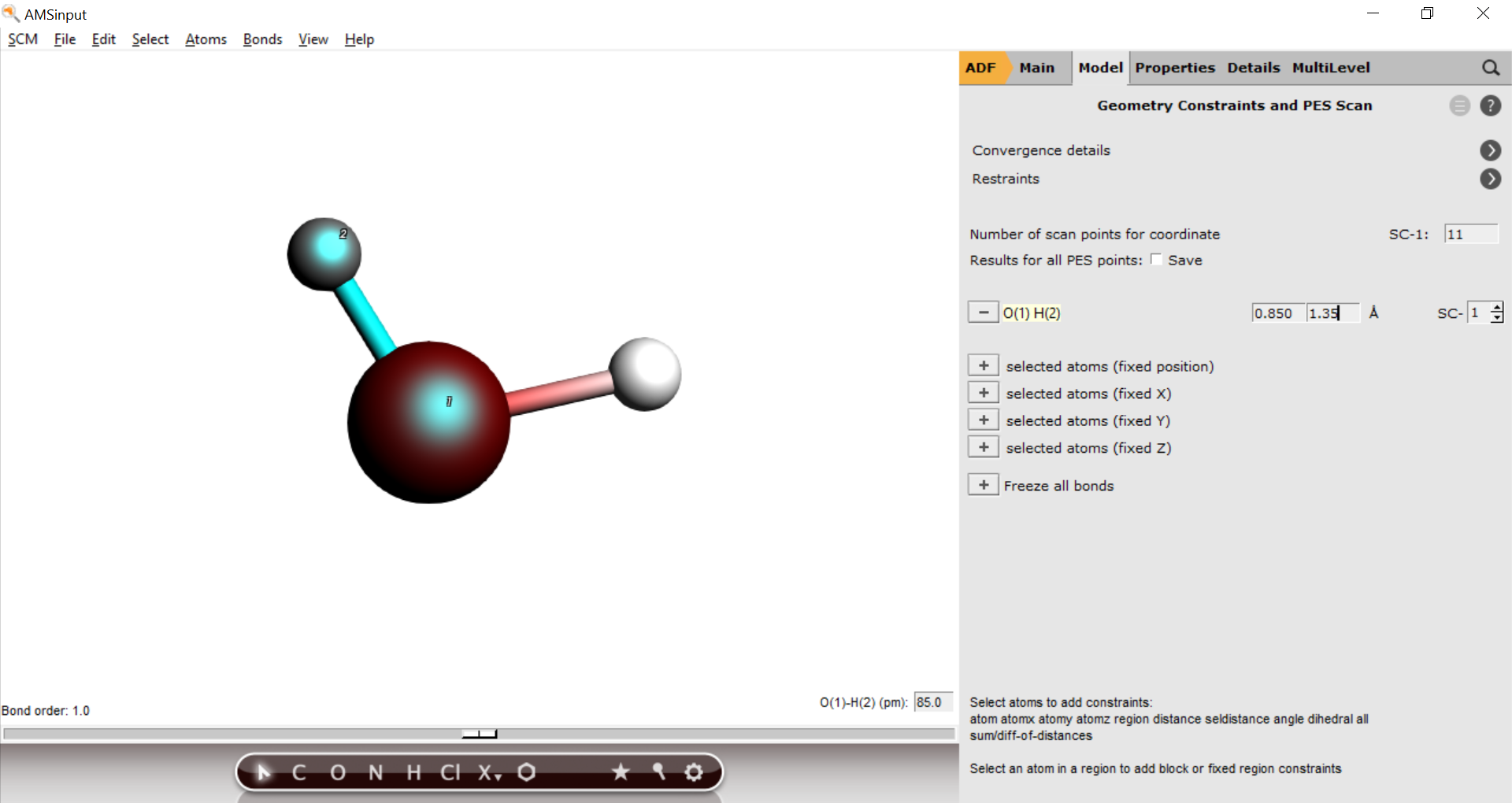
1. Open AMSinput with the ADF panel active. (If you do not have an ADF license, you can use a different reference engine).

2. Draw a water molecule, or use the search box to search for water

3. Task → PES Scan, and click the arrow icon to the right.

4. Select the O atom and one of the H atoms

5. Click the + icon next to O(1) H(2) distance

6. Set the number of scan points for SC-1 to 11

7. Set the range minimum to 0.85 angstrom, and the maximum to 1.35 angstrom.

8. Save with the name H2O_pesscan and run

From generate_input_files.py

def run_reference():
    # choose a reference engine. If you do not have a license for ADF, use DFTB, ForceField, or another engine for which you have the license.
    # from_smiles('O') creates an H2O molecule
    job = AMSJob.from_input(name='H2O_pesscan', molecule=from_smiles('O'), text_input='''
    Task PESScan
    PESScan
        # Scan O-H bond length between 0.85 and 1.35 angstrom (11 points)
        ScanCoordinate
            nPoints 11
            Distance 1 2 0.85 1.35
        End
    End
    Engine ADF
        XC
            GGA PBE
        End
    EndEngine
    #Engine ForceField
    #EndEngine
    #Engine DFTB
    #EndEngine
    ''')
    job.run()
    return job

First a Job Collection is defined, which also includes specifying the reference engine settings. The job is added as a job collection entry. From run.py

def create_job_collection():
    # Create a Job Collection, holding all jobs needed for the parametrization:
    jc = JobCollection()
    # Create a single Job Collection Entry with a H2O system:
    jce = JCEntry(molecule=from_smiles('O'))
    # The task is a PESScan with a H-O bond stretch, ranged [0.85, 1.35] angstrom:
    jce.settings.input.ams.task = 'pesscan'
    pes_points = np.linspace(0.85, 1.35, 11)
    jce.settings.input.ams.pesscan.scancoordinate.npoints = len(pes_points)
    jce.settings.input.ams.pesscan.scancoordinate.distance = f"1 2 {pes_points[0]} {pes_points[-1]}" # atom1 atom2 start end
    # Add the Entry to the Collection:
    jc.add_entry('water', jce)

    return jc, pes_points

Then the job collection is run with some given reference engine settings for the PBE functional:

def run_reference_calculations(jc : JobCollection):
    # The data set is missing reference values. Lets calculate them with PBE:
    pbe = Settings()
    pbe.input.adf.xc.gga = 'pbe'
    # Run all jobs in the Job Collection with the same settings:
    print('Running the reference calculation. This will take a moment ...')
    results = jc.run(pbe)

    return results

The JobCollection.run() function is also used by the $AMSBIN/params genref command (see ParAMS Main Script).

2.5.2. Import the reference data into ParAMS

GUI

Python

Detailed Python

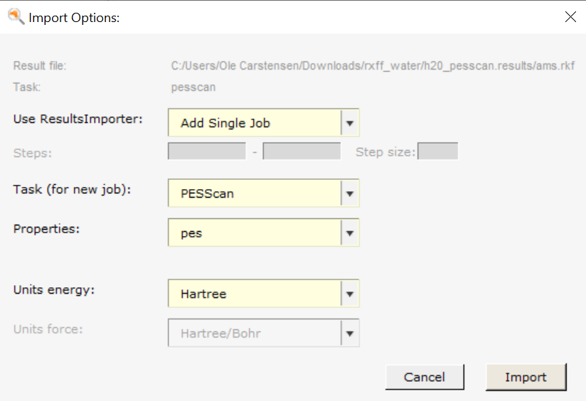
Select the finished reference job in AMSjobs

Job → Add to ParAMS (Ctrl-T)

This brings up the ParAMS GUI and an import dialog

In the dialog, set Use ResultsImporter to Add Single Job (default)

Set Task (for new job) to PESScan (default)

Set Properties to pes (default)

Click Import

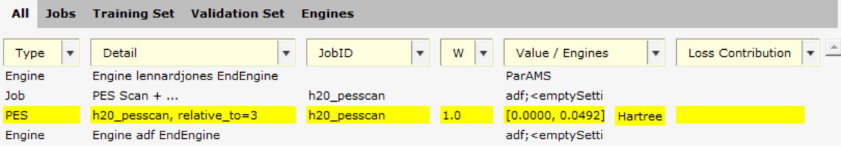
This adds

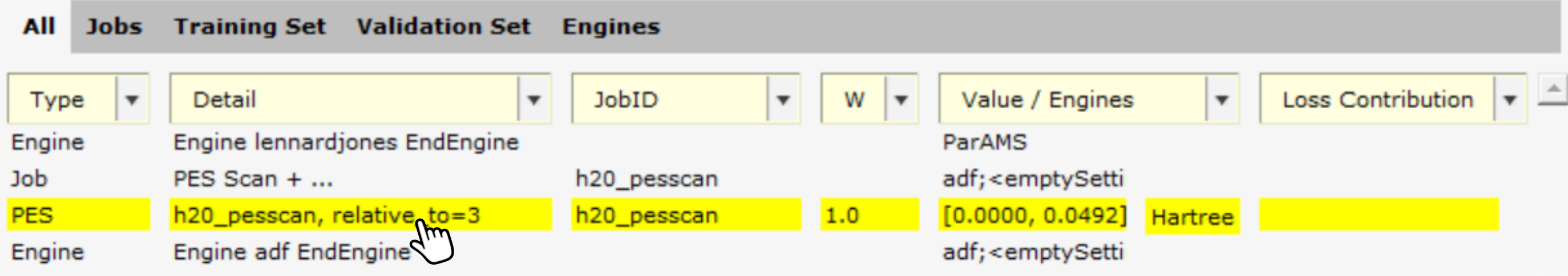
• A job with the ID H2O_pesscan to the Job Collection. It has task PESScan, with settings taken from the reference pes scan job (which bond to scan, the number of points to sample, etc.).
• A training set of type PES with the detail H2O_pesscan, relative_to=3. The relative_to_3 means that the energies along the bond scan are calculated with respect to the 4th point (the indexing starts with 0), because that point was the lowest in energy. Select the entry and switch to the Info panel at the bottom to see the reference values.
• An engine adf;;xc;;gga;PBE;. This engine contains the settings that were used in the reference calculation.

If you would like to change the point along the bond scan that the other energies are relative to, it can be done as follows:

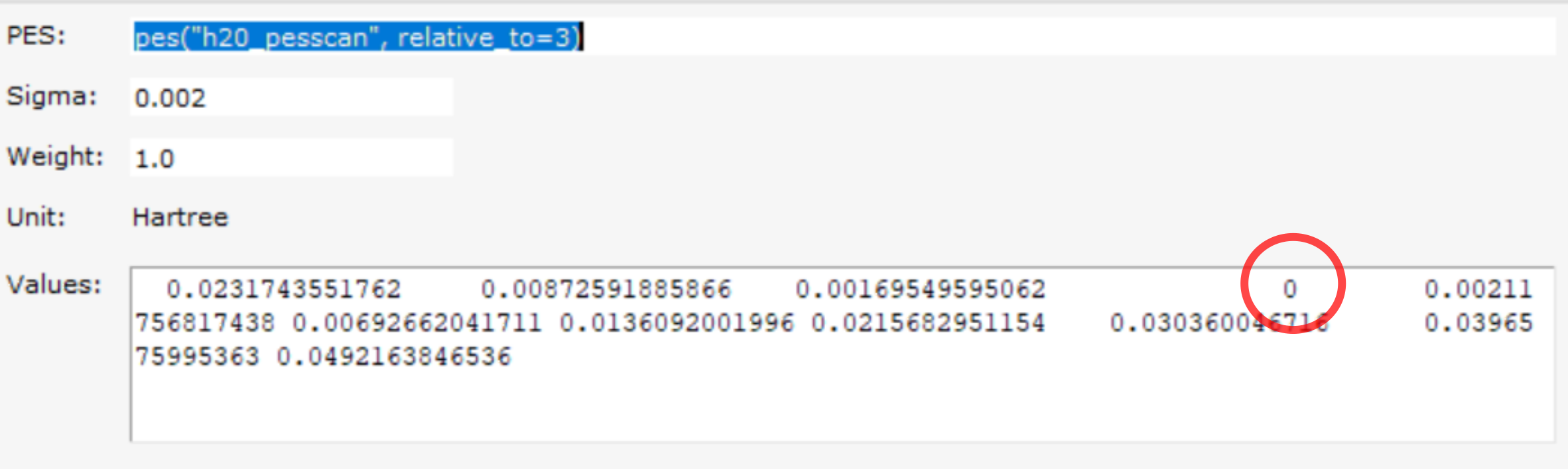
Go to the Training Set panel

Double-click in the Details column where it says H2O_pesscan, relative_to=3. This brings up a dialog with more details.

Note how the 4th value is 0.0 and all the other numbers are positive

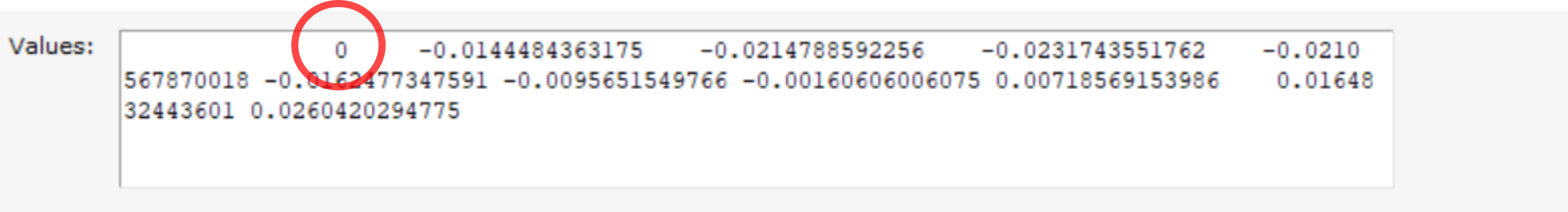
On the PES line, change relative_to=3 to relative_to=0.

Click OK. Note: The reference values have not yet changed!

Select the entry on the Training Set panel.

Training Set → Get Data From Ref Jobs

This updates the reference values.

Double-click in the Details column where it says H2O_pesscan, relative_to=0. This brings up a dialog with more details.

Note how the 1st value is now 0.0, and some of the other numbers are negative

Change back: On the PES line, change relative_to=0 to relative_to=3.

Select the entry on the Training Set panel.

Training Set → Get Data From Ref Jobs

This updates the reference values.

See also

Import training data (GUI)

From generate_input_files.py. The following lines set up a Results Importer with kcal/mol energy units, import the results, and store the training_set.yaml and job_collection.yaml files. It also illustrates the use of a weights scheme, in which the weights depend on the reference values. Run the script with $AMSBIN/amspython generate_input_files.py.

def import_results():
    # If you ran the PESScan job via the graphical user interface, set
    #pesscan_job = '/path/to/ams.rkf'
    # Otherwise, the below line runs the reference job
    pesscan_job = run_reference()
    ri = ResultsImporter(settings={'units': {'energy': 'kcal/mol'}})
    ri.add_singlejob(pesscan_job, task='PESScan', properties={
        'pes': {
            # apply a weights scheme (optional). 
            # This sets the weight for the larger energies (very short or very long bond distance) to smaller numbers.
            # stdev is the standard deviation of the Gaussian in energy units (here kcal/mol)
            'weights_scheme': WeightsSchemeGaussian(normalization=11.0, stdev=20.0)
        }
    })
    ri.store(binary=False, backup=False, store_settings=False)

See also

Import training data (Python)

From run.py. A training set (Data Set) is created:

def create_training_set():
    # Define the training set. Here, we will just add one entry: The PES of the H-O bond scan of water:
    ds = DataSet()
    ds.add_entry("pes('water')")
    return ds

The reference values are set from the results returned by run_reference_calculations:

def update_training_set_with_reference_results(ds : DataSet, results : dict):
    # Extract the relevant results and populate all reference values in the Data Set:
    ds.calculate_reference(results)

2.5.3. Set the parameters to optimize

In this case, we will optimize all O-H bond parameters of the ReaxFF force field. The starting point (initial parameters) come from Water2017.ff (DOI: 10.1021/acs.jpcb/7b02548).

GUI

Python

Detailed Python

First, load Water2017.ff:

In the ParAMS GUI, select Parameters → Load ReaxFF Force Field → Water2017.ff

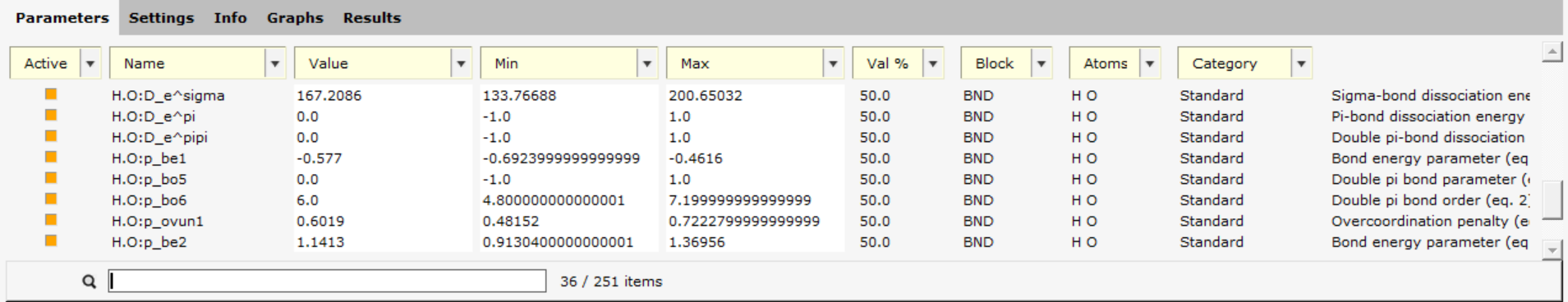
Next, only set the O-H bond parameters to be active:

Switch to the Parameters tab in the bottom half

In the Block drop-down, choose BND (bond parameters)

In the Category drop-down, choose Standard - these are the parameters that are most common to optimize.

Scroll down to the bottom, and tick the Active checkbox for all 12 parameters with Atoms equal to H O

Tip

In the bottom search box, type H.O: to search for parameters between H and O (both BND and OFD parameters). Remember to clear the search box to see all parameters again.

Note

Normally you wouldn’t optimize all bond parameters, but only a few of them (you could try different combinations). Here, we optimize all bond parameters for illustration purposes only. For example, optimizing π-bond parameters for H₂O is not very useful!

See also

The equations that the parameters enter.

From generate_input_files.py. The following function initializes a ReaxFF Parameter interface based on the parameters in Water2017.ff.

• bounds_scale=1.2 means that the minimum and maximum allowed values will be within 20% of the original value for all optimized parameters.
• header['head'] is the first line of the output ffield.ff (force-field) file
• Only the O-H bond parameters become active.
• The interface is stored in the file parameter_interface.yaml.

def create_parameter_interface():
    # start from the Water2017.ff force field
    parameter_interface = ReaxFFParameters('Water2017.ff', bounds_scale=1.2)
    parameter_interface.header['head'] = "Reparametrization of Water2017.ff"
    # only activate the "Standard" bond parameters for O-H
    for p in parameter_interface:
        p.is_active = (p.metadata['block'] == 'BND') and \
                      (p.metadata['category'] == 'Standard') and \
                      (p.metadata['atoms'] == ['H', 'O'] or p.metadata['atoms'] == ['O', 'H'])
    parameter_interface.yaml_store('parameter_interface.yaml')

From run.py. The following function initializes a ReaxFF Parameter interface Only the O-H bond parameters become active.

def create_parameter_interface():
    # Load the ReaxFF force field we want to optimize:
    parameter_interface = ReaxFFParameters('Water2017.ff')
    # First line of the output ffield.ff file
    parameter_interface.header['head'] = "Reparametrization of Water2017.ff"
    # Mark only parameters from the H-O Bonds block for optimization:
    for parameter in parameter_interface:
        parameter.is_active = parameter.metadata['block'] == 'BND' and \
                              (parameter.metadata['atoms'] == ['H', 'O'] or parameter.metadata['atoms'] == ['O', 'H'])

    return parameter_interface

2.5.4. Run the ReaxFF parametrization

For ReaxFF, we recommend to use the CMA-ES Optimizer. It is a method which samples popsize parameters around a central point (mean). The first central point is the initial parameters. The sigma keyword affects how broad the sampled distribution is (how far away from the central point parameters are sampled).

After an iteration, which consists of popsize parameter evaluations, the central point and sigma are updated. The central point will approach the optimized parameters, and sigma will decrease as the optimization progresses. In this way, the sampled distribution is very broad in the beginning of the optimization, but becomes smaller with time.

When sigma reaches the minsigma value, the optimization stops.

See also

• Video tutorial on YouTube about CMA-ES with ReaxFF (AMS2021 version)
• How to restart/continue CMA-ES optimizations

Tip

Decrease the initial sigma value for faster convergence (less global optimization).

GUI

Python/Command-line

Detailed Python

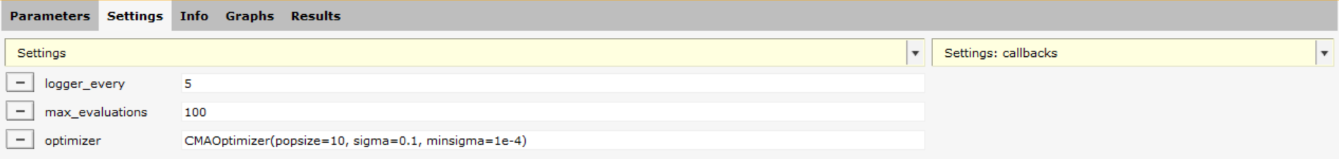
Switch to the Settings tab in the bottom table

In the dropdown, choose Optimizer: CMAOptimizer.

On the optimizer line, set popsize to 10, sigma to 0.1, and minsigma to 1e-4

In the dropdown, choose Max Evaluations

Set max_evaluations to 100

In the dropdown, choose Logger

Set logger_every to 5

File → Save As

Save with the name reaxff_water.params

File → Run

The params.conf.py file contains:

optimizer = CMAOptimizer(popsize=10, sigma=0.1, minsigma=1e-4)

max_evaluations = 100

logger_every = 5

• optimizer = CMAOptimizer(popsize=10, sigma=0.1, minsigma=1e-4) initializes a CMAOptimizer
• max_evaluations = 100 means that the optimization will stop after 100 evaluations.
• logger_every = 5 means that logging will happen every 5 evaluations or whenever the loss function decreases

To run the optimization:

"$AMSBIN"/params optimize

From run.py.

def run_optimization(jc : JobCollection, ds : DataSet, pi : ReaxFFParameters):
    # Choose an optimization algorthm:
    o = CMAOptimizer(sigma=0.1) # sigma range: (0, 1). smaller sigma -> more local sampling

    # Piece it all together and run:
    O = Optimization(
        job_collection=jc,
        data_sets=ds,
        optimizer=o,
        parameter_interface=pi,
        callbacks=[MaxIter(100)], # The MaxIter callback stops an optimization after N evaluations
        )
    O.optimize()
    return O

2.5.5. Visualize the results

For more details about graphs and results, see the Getting Started: Lennard-Jones Potential for Argon tutorial.

GUI

Command-line

Detailed Python

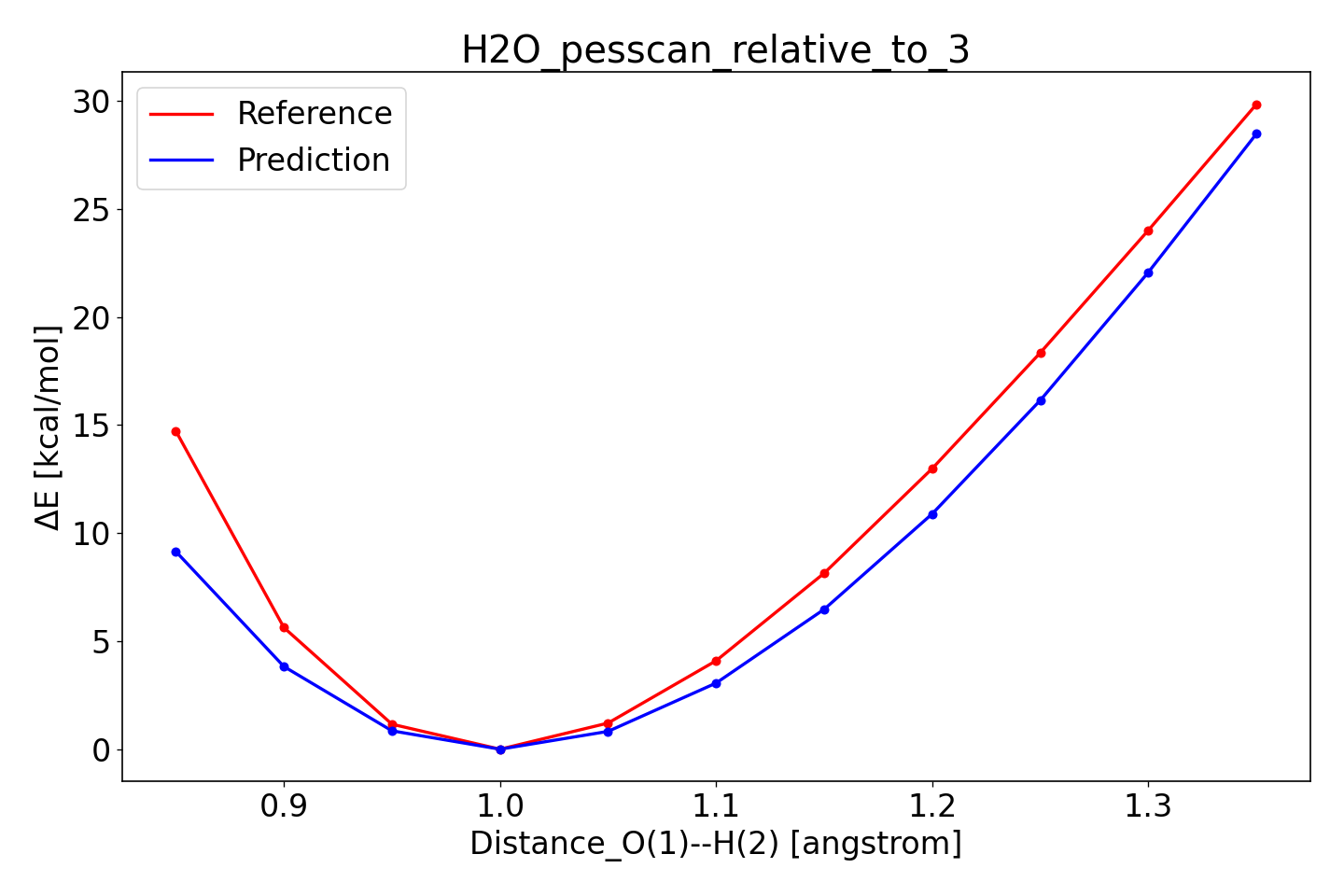
On the Graphs tab, select Best H2O_pesscan_relative_to_3.

This plots the file optimization/training_set_results/best/pes_predictions/H2O_pesscan_relative_to_3.txt.

To compare to the bond scan using Water2017.ff, choose Data From → Training(initial): ΔE_prediction.

Tip

You double-click on a plot axis to access plot configuration settings.

In the directory optimization/training_set_results/best/pes_predictions, there is a file H2O_pesscan_relative_to_3.txt. The relative_to_3 means that the energies along the bond scan are calculated with respect to the 4th point (the indexing starts with 0). Use params plot H2O_pesscan_relative_to_3.txt to generate an image like the following:

To compare to the initial parameters, make the corresponding plot from the optimization/training_set_results/initial/pes_predictions directory.

From run.py.

def create_plots(workdir, pes_points):
    # At this point the optimization is done.
    # All relevant optimization data is stored in `O.workdir`
    # Data with the best parameters is stored in `training_set_results/best`
    # For more information on what is logged, refer to the `Logger()` callback documentation
    # Lets visualize some of it:
    from os.path import join as opj
    import matplotlib.pyplot as plt

    initial_ffield_ds     = DataSet( opj(workdir, 'training_set_results', 'initial', 'data_set_predictions.yaml') )
    initial_predictions   = initial_ffield_ds["pes('water')"].metadata['Prediction']
    optimized_ffield_ds   = DataSet( opj(workdir, 'training_set_results', 'best', 'data_set_predictions.yaml') )
    optimized_predictions = optimized_ffield_ds["pes('water')"].metadata['Prediction']
    reference             = initial_ffield_ds["pes('water')"].reference

    plt.rcParams['font.size'] = 16
    plt.figure(figsize=(8,6))
    plt.plot(pes_points, 2.6255e+03*reference, color='k', label='Reference') # convert hartree to kj/mol
    plt.plot(pes_points, 2.6255e+03*initial_predictions, label='Initial FF')
    plt.plot(pes_points, 2.6255e+03*optimized_predictions, label='Optimized FF')
    plt.ylabel('ΔE [kJ/mol]')
    plt.xlabel('H-O distance [Å]')
    plt.legend()
    plt.savefig('pes_results.png')

2.5.6. ffield.ff: The force field file

To run new ReaxFF simulations with your fitted force field, you need the force field file ffield.ff.

You can find it in the results directory in optimization/training_set_results/best/ffield.ff.

Tip

The first line of the file is a header. Fill it with some meaningful content describing

• who made it,
• when it was made, and
• the types of training data (systems, reference methods)

You can also change the header in the ParAMS GUI: Select Parameters → Edit ReaxFF header before running your job.

2.5.7. Summary of the 3 different ways

Differences of the three different ways of running this tutorial (GUI, Python/Command-line, and Detailed Python) are given below:

Action	GUI	Python/Command-line	Detailed Python
Run reference job	AMSinput/AMSjobs	PLAMS	JobCollection.run()
Import results	Import dialog	Results Importer	DataSet.calculate_reference()
Set max evaluations	Settings: max_evaluations 100	max_evaluations = 100 in params.conf.py	callbacks=[MaxIter(100)] in the Optimization constructor
Final plot	Graphs panel	xy file auto-generated (params plot)	Python code

2.5.8. Next steps with ReaxFF parametrization

Check out the ReaxFF: Adsorption on ZnS(110) for a more realistic parametrization, which also shows how to build a new ReaxFF force field from scratch.