Silicon Gate Oxide Characterization with XPS

BAND Semiconductors Spectroscopy XPS

Gate oxide nitrisation is employed in CMOS processing to increase material capacitance, allowing for smaller components to be manufactured. Nitrogen dosing needs to be balanced however, as nitrogen diffusion into the channel can cause trapping, leading to reduced transistor lifetimes.

To assure uniform wafer properties, angle-resolved X-ray photoelectron spectroscopy (ARXPS) is used to probe the nitrogen profile throughout the gate thickness. Deconvolution of these XPS spectra subsequently relies on accurate reference data on the chemical shifts, which are dependent on the local composition along the gate profile.

This tutorial will showcase the prediction of Si(2p) XPS spectra for various SiO_xN_y phases. The predicted phase shifts are used to analyze trends in experimental ARXPS spectra, illustrating the application of this workflow in semiconductor metrology.

Note

In order to obtain accurate predictions for XPS spectra, DFT calculations will be performed on extended systems. These calculations may take 8-12 hours on a 32 core system. You can choose to skip these calculations and only focus on the instructions provided for small systems when learning how to perform XPS calculations with BAND.

XPS Procedure

We will start by illustrating the basic procedure for XPS calculations for pure Silicon. The Δ-SCF method will be used in order to obtain the core electron binding energy relative to the valance band maximum (VBM).

\[E_b(j) = E_h^{N-1}(j) - E_h^{N-1}(\textrm{VBM})\]

This will require us to perform 2 calculations:

• Determine the energy of the core-hole state

• Determine the reference energy for the VBM-hole state

Note

Using the Fermi level as the reference state makes experimental comparison more difficult as its position is highly sensitive to the presence of sample impurities, leading to higher uncertainties. The VBM reference meanwhile remains static, and is considered the preferred approach when evaluating XPS binding energies for solids.[1]

Si(2p) Binding Energy in Si

The starting point for an XPS calculation is the minimum-energy structure of the solid compound. For Si, we can retrieve the coordinates from the built-in database.

1. Start AMSinput: SCM → New Input

2. In the menu, type Si and select the Si crystal structure

AMSinput will automatically switch to the BAND engine when a solid structure is selected. We will now configure the settings for the VBM-hole calculation:

1. Select XC functional → MetaGGA → SCAN. The SCAN meta-GGA functional has been reported to provide high accuracy for XPS binding energies,[1] and will therefore be used here

2. Set Total charge to 1. This removes 1 electron from the system

3. Enable Unrestricted calculations because we now have an unequal number of alpha and beta electrons

4. Set Spin polarization to 1. This forces the solution to have an excess alpha electron. For Δ-SCF, it is important that both the core-hole and VBM-hole excitation target the same spin

5. Set Basis set to TZP. This provides good accuracy for inorganic solid structures, and we do not need to resort to a more expensive TZ2P basis

6. Save the input using File → Save as with the name Si_VBM

7. Start the simulation using File → Run

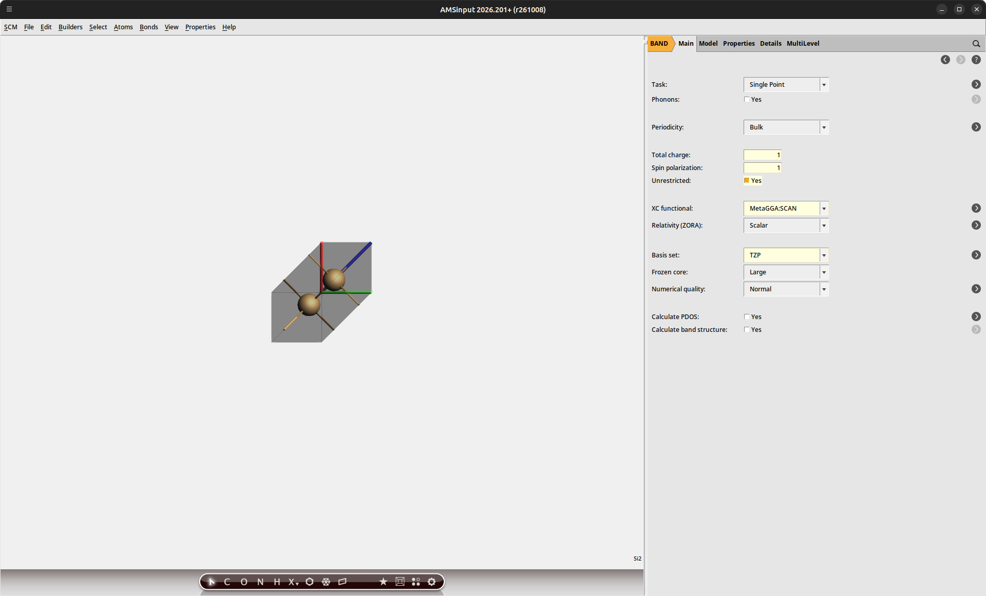
For the core-hole excitation, we additionally need to specify which core electron will be excited. The core states in our structure are ordered by ascending energy. Because our unit cell contains 2 Si atoms, we select the 5th orbital in order to determine the Si(2p) state.

Band	Atom	Core orbital
1	Si(1)	Si(1s)
2	Si(2)	Si(1s)
3	Si(1)	Si(2s)
4	Si(2)	Si(2s)
5	Si(1)	Si(2p)

1. Set Frozen core to None. This will allow us to perform a core excitation

2. Because we are exciting a p-electron, this will break the symmetry of the system. Go to Details → Symmetry and disable the Use symmetry option.

3. Go to Model → Spin and Occupation. For the Electron hole set the Band index to 5 and the Spin index to 2. This will excite the beta electron from the Si(2p) core state

4. Save the input using File → Save as with the name Si_CH_5b

5. Start the simulation using File → Run

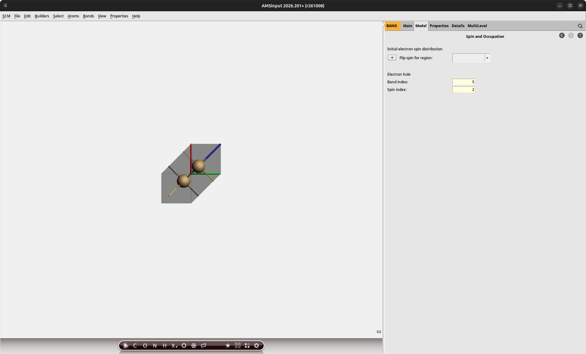
By performing an SCF calculation on the core-hole state, our calculations will explicitly include the relaxation of the electronic structure in the presence of the hole. Once both calculations have finished, we can extract the energy using AMSoutput.

1. Go to AMSjobs: SCM → Jobs

2. Select a calculation and open SCM → Output

3. Go to AMS → Energy to find the required system energy value

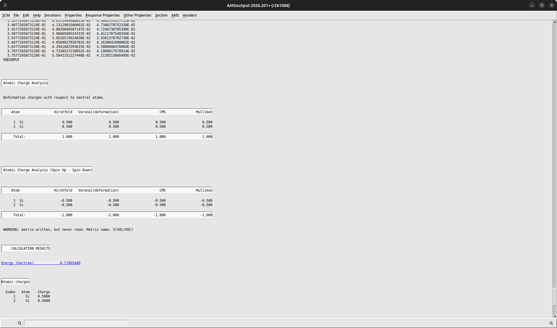
We can collect the results of our calculations here:

Variable	Energy (Ha)	Energy (eV)
\(E_h^{N-1}(\textrm{VBM})\)	-0.1787	-4.86
\(E_h^{N-1}(5)\)	3.4046	92.64
\(E_b\)	3.5832	97.51

This initial result produces quite a poor estimate for the XPS binding energy resulting from the use of a small periodic unit cell. This effectively increases the hole density, resulting in hole-hole interactions across the system. In order to obtain accurate predictions for the binding energies, it is required to obtain our data in the limit of isolated holes.

Supercell Convergence

The central approach is to repeat our calculation for a larger supercell, from which we can then extrapolate the limiting values.

1. Start AMSinpu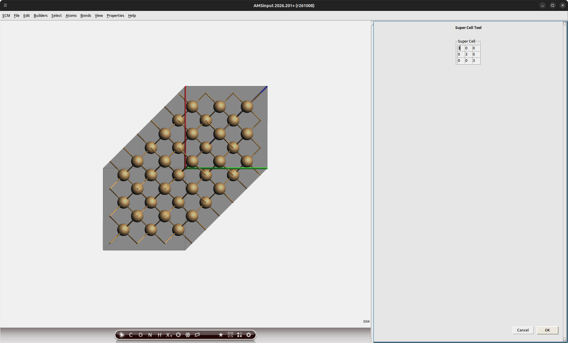t: SCM → New Input

2. Use File → Open to load our Si bulk structure from Si_VBM

3. Go to Edit → Crystal → Generate Supercell. Change the diagonal values to 3 and click OK to generate the extended supercell

4. Save the input using File → Save as with the name Si_333_VBM

5. Start the simulation using File → Run

Note

The recommended approach would be to perform a linear interpolation between energies obtained for 1x1x1, 2x2x2 and 3x3x3 cells. A 1x1x1 calculation can sometimes fall outside of the linear regime, particularly when small unit cells are used. Visual inspection of the energies is recommended to confirm that the linear extrapolation approach is valid. Datapoints for unit cells larger than 3x3x3 are seldom needed.

Because the number of atoms in our cell has increased, the band index for the core-hole state must be adapted as well.

1. Set Frozen core to None.

2. Go to Details → Symmetry and disable the Use symmetry option.

3. Go to Model → Spin and Occupation and set the Band index to 109 and the Spin index to 2.

4. Save the input using File → Save as with the name Si_333_CH_109b

5. Start the simulation using File → Run

The binding energies obtained from supercell calculations of 2x2x2 and 3x3x3 cells are shown in the figure below. The extrapolation towards the limit of the isolated hole is highlighted visually.

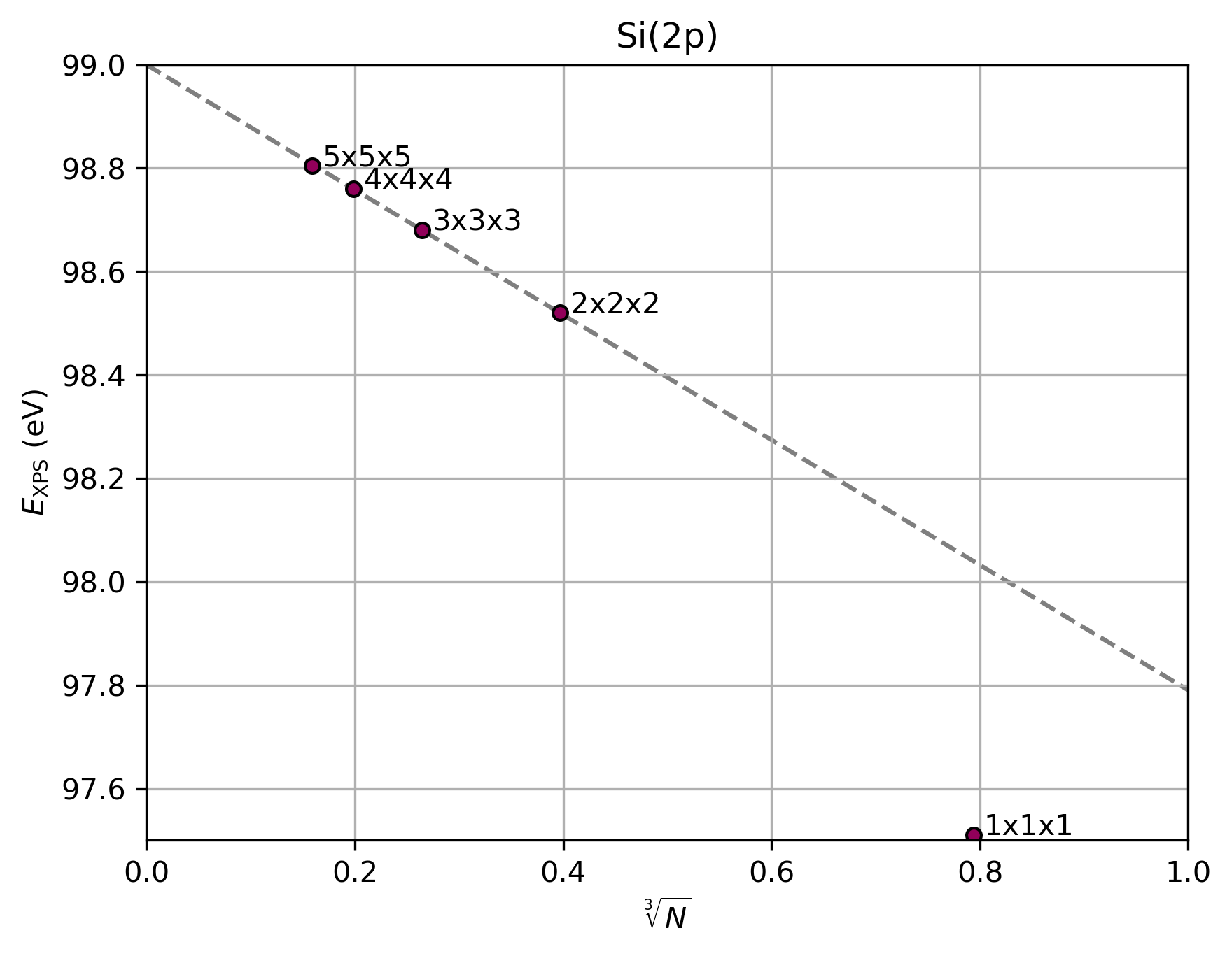
Fig. 73 Si(2p) binding energies predicted using BAND for different unit cell sizes. The grey line indicates a linear fit through the 2x2x2 and 3x3x3 data

We can see that the results for the 1x1x1 cell fall outside the linear extrapolation regime due to the high effective hole density in the small cell. We therefore make use of the 2x2x2 and 3x3x3 cells to perform the extrapolation to the limit of the isolated hole.

\[E_{N\downarrow{0}} = E_\mathrm{3x3x3} - N_\mathrm{3x3x3} \frac{ E_\mathrm{3x3x3} - E_\mathrm{2x2x2} }{ \sqrt[3]{N_\mathrm{3x3x3}} - \sqrt[3]{N_\mathrm{2x2x2}} }\]

Where \(N\) denotes the number of atoms in each supercell.

Variable	Energy (eV)
\(E_b(\textrm{1x1x1})\)	97.51
\(E_b(\textrm{2x2x2})\)	98.52
\(E_b(\textrm{3x3x3})\)	98.68
\(E_b(N\downarrow{0})\)	99.00

The resulting binding energy now fully matches the experimental value[2] of 99.03 eV (to within the accuracy of DFT). A brief comparison between the values predicted from the individual cell calculations highlights the importance of evaluating the isolated hole limit.

Si(2p) Binding Energy in SiO_xN_y

We can extend our study towards other SiO_xN_y phases in order to provide reference data for interpreting experimental spectra. We will consider both SiO₂ and Si₂N₃ phases as saturation points for the binary compositions. The intermediate Si₃O₅N₁ and Si₃O₄N₂ compositions will be evaluated to show the shift in binding energy with increased nitrogen content.

• The SiO₂ structure is available in the AMSinput database under the name AlphaQuartz.

• The Si₂N₃ structure can also be loaded from the database directly.

• The Si₃O₅N₁ structure can be made by substituting one of the oxygen atoms in the SiO₂ structure with nitrogen. (Using Atoms → Change atom type in AMSinput.)

• The Si₃O₄N₂ structure can be made by substituting one of the oxygen atoms in the Si₃O₅N₁ structure with nitrogen.

For each of these phases, we repeat the XPS procedure outlined before:

• Perform the VBM-hole calculation for the 2x2x2 supercell

• Perform the VBM-hole calculation for the 3x3x3 supercell

• Perform the core-hole calculation for the 2x2x2 supercell

• Perform the core-hole calculation for the 3x3x3 supercell

The results of these calculations have been summarized in the figure below.

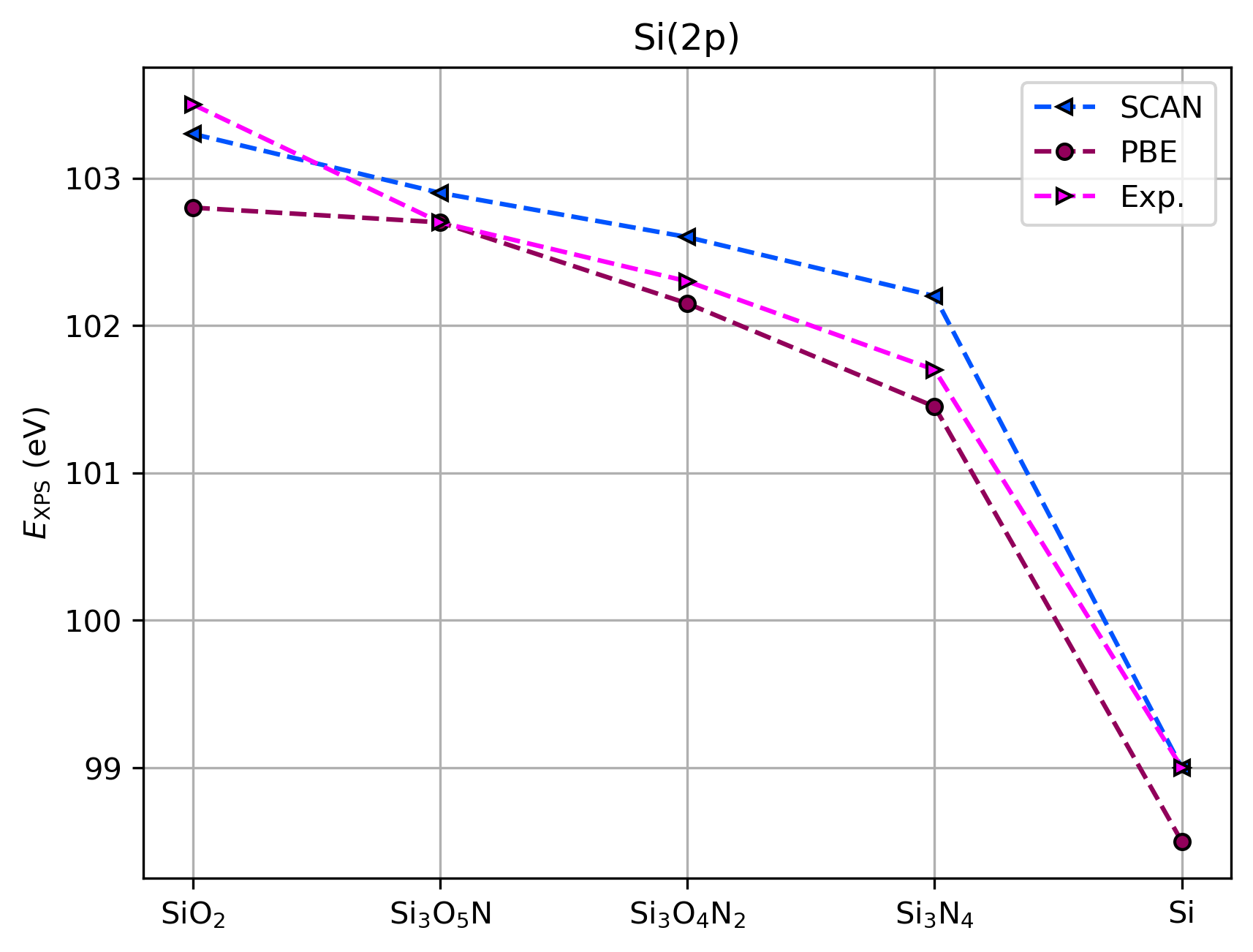
Fig. 74 Comparison between experimental XPS binding energies[2] and Δ-SCF predictions using BAND

Phase	\(E_b^{calc}\) (eV)	\(E_b^{exp}\) (eV)
SiO2	103.3	103.5
Si3O5N1	102.9	102.7
Si3O4N2	102.6	102.3
Si2N3	102.2	101.7
Si	99.0	99.0

Good agreement with experimental values is obtained. With increasing nitrogen content, we see a shift in the XPS signal towards lower binding energy, following the decreased electronegativity relative to oxygen. The values obtained at different nitrogen content levels can be correlated to experimental ARXPS measurements to determine the nitrogen profile inside a plasma-treated gate oxide.[2] Because the chemical shifts are dependent on the phase, characterization of the dominant crystal structures inside the gate can also be performed.

The high accuracy of the XPS binding energy calculations provides a reasonable level of confidence in predictive modeling strategies. 2 key aspects should however be considered:

• Extrapolation towards the isolated hole limit must be performed in order to obtain reliable estimates for XPS binding energies in solids

• Peak distances between different core signals will exhibit higher errors, as the DFT prediction error is not one-sided. E.g. the SiO₂ binding energy is slightly overestimated, while Si₂N₃ is slightly underestimated

See also

Spin-orbit coupling, responsible for peak splitting in XPS spectra, was not considered in the current tutorial as the doublet splitting for Si(2p) is less than the typical accuracy range of DFT, and can therefore not be disambiguated.

For other systems, such as HfO₂, this effect is much greater and should be considered in the calculations. This is easily achieved by enabling the Relativity → Spin-Orbit option in AMSinput.

References

[1] (1,2)

J. M. Kahk, G. S. Michelitsch, R. J. Maurer, K. Reuter, J. Lischner, Core Electron Binding Energies in Solids from Periodic All-Electron Δ-Self-Consistent-Field Calculations. J. Phys. Chem. Lett. 12, 9353-9359 (2021)

[2] (1,2,3)

C. R. Brundle, G. Conti, P. Mack, XPS and Angle Resolved XPS in the Semiconductor Industry: Characterization and Metrology of Ultra-Thin Films. J. Electron Spectrosc. 178-179, 433-448 (2010)