Microkinetics: CO Oxidation
In this tutorial we will walk you through example microkinetic calculations with the program MKMCXX, using the GUI.
- When you publish results in the scientific literature which were obtained with the MKMCXX program you should include the following reference:
Ivo A. W. Filot, Prof. Dr. Rutger A. van Santen, Prof. Dr. Emiel J. M. Hensen, The Optimally Performing Fischer–Tropsch Catalyst, Angew. Chem. Int. Ed., 53: 12746-12750 (2014)
See also
In the conversion from reagents to their final product(s), often many smaller intermediate steps are involved. These elementary reaction steps have each their individual energy barriers and rate constants, the combination of which yields the overall reaction system behavior. Via microkinetic modeling such a system can be investigated, yielding information on reaction rates and rate-limiting factors.
From a set of elementary reaction steps, MKMCXX automatically sets up and solves a system of differential equations. The following features are present:
Calculating the reaction rate over a range of temperatures
Calculating the selectivity between different products
Determining the reaction orders and apparent activation energies of the reaction
Calculating the degree of rate control for all reaction steps
Handle homogeneous and heterogeneous reactions
Apply a well-mixed or plug-flow reactor
Modeling Temperature Programmed Desorption
Modeling isotopic switches
In this tutorial we will study the CO oxidation reaction on a catalyst. Here, we will determine the temperature corresponding to the maximum reaction rate, as well as the dependence of the reaction rate on the partial pressure of the reagents.
In CO oxidation, the reagents CO and O2 are converted to CO2. 4 individual reaction steps can be identified: The adsorption of CO, O2, and CO2, and the surface reaction from adsorbed O and CO to CO2. The energy barriers for the reaction steps can be calculated beforehand by a Transition State calculation via DFT.
Step 1: Specify compounds
The MKMCXX [1] input is specified in a different GUI module than usual: AMSkinetics.
The first step is to identify the compounds and reaction intermediates that may play a role in the reaction. They are split apart in two categories: Gas-phase compounds and adsorbed compounds. Gas-phase compounds are mobile and their concentration is controlled by their partial pressure. Adsorbed compounds are localized on the catalyst surface and compete for space. After starting up the GUI, the two compound tables are opened on the left-hand side of the window.
Entries can be added to the tables by pressing the  button in the top left corner. Alternatively, the right-click menu has an option to add multiple new rows at once. The values inside the tables can be edited by double-clicking, or by selecting a field and pressing
 Enter. By selecting cells inside the table, values can be copied and pasted. In this manner, values from other spreadsheets (such as Excel) can be easily copied over.
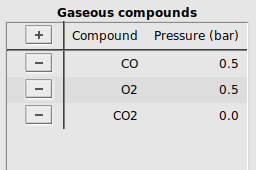
Every unique compound in the system has an entry in the compound tables. An entry specifies a label describing a compound, along with their initial concentration at the start of the simulation. In CO oxidation, three different gas-phase compounds are present: The reactants CO and O2, and the product CO2. We will take the initial situation with a 1:1 ratio of CO to O2, with no CO2.
buttonCompound to start editingCO (this will be the label for the CO molecule in our calculation)Pressure (bar), add the initial partial pressure of this compound, here 0.5O2 and CO2, with initial concentrations 0.5 and 0.0 respectivelyIt should look like this:
Next, the list of adsorbed compounds are specified. In MKMCXX all surface sites are equivalent to one another. The sum total coverage of all adsorbates on the surface is normalized to 1. To keep the reaction balances consistent, we specify an empty, free surface site *, which is consumed whenever another compound adsorbs to the surface site. CO adsorbs associatively, giving an adsorbed species which will be labeled as CO*. O2 adsorbs dissociatively, giving an adsorbed species which will be labeled as O*. The product that is formed will be labeled CO2*.
At the start of the simulation the surface will be free of adsorbates, meaning that only empty surface sites are present initially.
button*, CO*, O*, and CO2* labels to the column CompoundFraction, fill in 1.0 for * and 0.0 for the other compoundsIt should look like this:
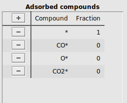
By specifying 1.0 for the empty surface site and 0.0 for all other adsorbed compounds, all surface sites are available at the start of the simulation.
Step 2: Specify reactions
The next step is to identify the reaction steps and adsorption/desorption steps. They are split apart in two categories: Hertz-Knudsen-type reactions and Arrhenius-type reactions. Arrhenius-type reaction equations are used most often with reactions occurring in the same phase, such as surface reactions or gas-phase reactions. However, they are not a good fit for adsorption/desorption steps, as they describe the transition from the mobile 3D gas phase to the restricted 2D surface poorly. For these types of steps, Hertz-Knudsen-type steps are preferred. After starting up the GUI, the two reaction tables are opened in the middle of the window. Different variants of reaction equations can be specified by switching to a different tab.
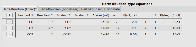
To allow the reactants CO and O2 to adsorb to the surface, and the product CO2 to desorb, we will specify three adsorption/desorption steps. We will use the tab Hertz-Knudsen (linear), as all these three molecules are linear.
buttonCO and * to the reactant columns, and CO* to the product columnsO2 and 2 * to the reactant columns, and 2 O* to the product columnsCO2 and * to the reactant columns, and CO2* to the product columns[1e-20, 28, 2.8, 1, 1, 80e3][1e-20, 32, 2.1, 2, 1, 40e3][1e-20, 44, 0.56, 1, 1, 10e3]It should look like this:
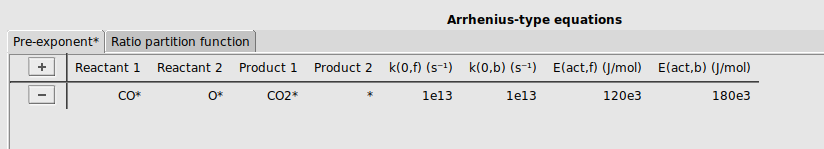
Finally, we will specify a reaction between adsorbed CO* and O* to form CO2*.
buttonCO* and O* to the reactant columns, and CO2* and * to the product columns.[1e13, 1e13, 120e3, 180e3]It should look like this:
With these two steps, we have specified all participating compounds and reaction intermediates in the system, as well as how they are connected into a reaction network.
Step 3: Specify properties to calculate
In the final step for setting up the simulation, we will select the simulation mode as well as the properties of the reaction network to calculate. After starting up the GUI, the simulation settings are found in the right-most panel.
In this example calculation, we will determine the overall reaction rate and the reaction order of each of the reactants, for a range of temperatures.
DefaultTotal pressure field empty to the right of
 Temperature run(s)300 to 800 K.25 K.Calculate: Orders to the right of Orders buttonCO and O2 buttonCO2At this moment, all the required information has been specified to run the simulation.
Step 4: Run and analyze results
To run the simulation, press the Run button found at the bottom right of the notebook. Alternatively, in the menu bar, select File → Run. This will open up AMSjobs, if it hasn’t yet been opened. The calculation will now run.
The simulation results are printed out in the folder results. A summary of the final state of each temperature run is put into the run/range subfolder. If the box next to Create graphs was checked in the Output Details (true by default), additional plots are created in .pdf format in the run/graphs subfolder. This allows for a quick inspection of the simulation results. These plots can be opened from AMSjobs by double-clicking the name in the results folder.
The resulting plots will look similar to this:
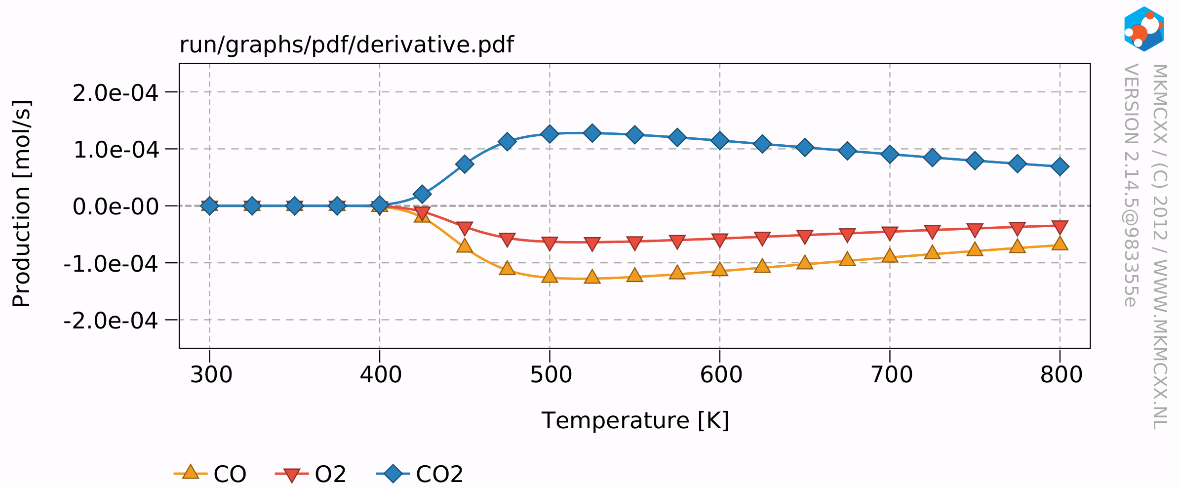
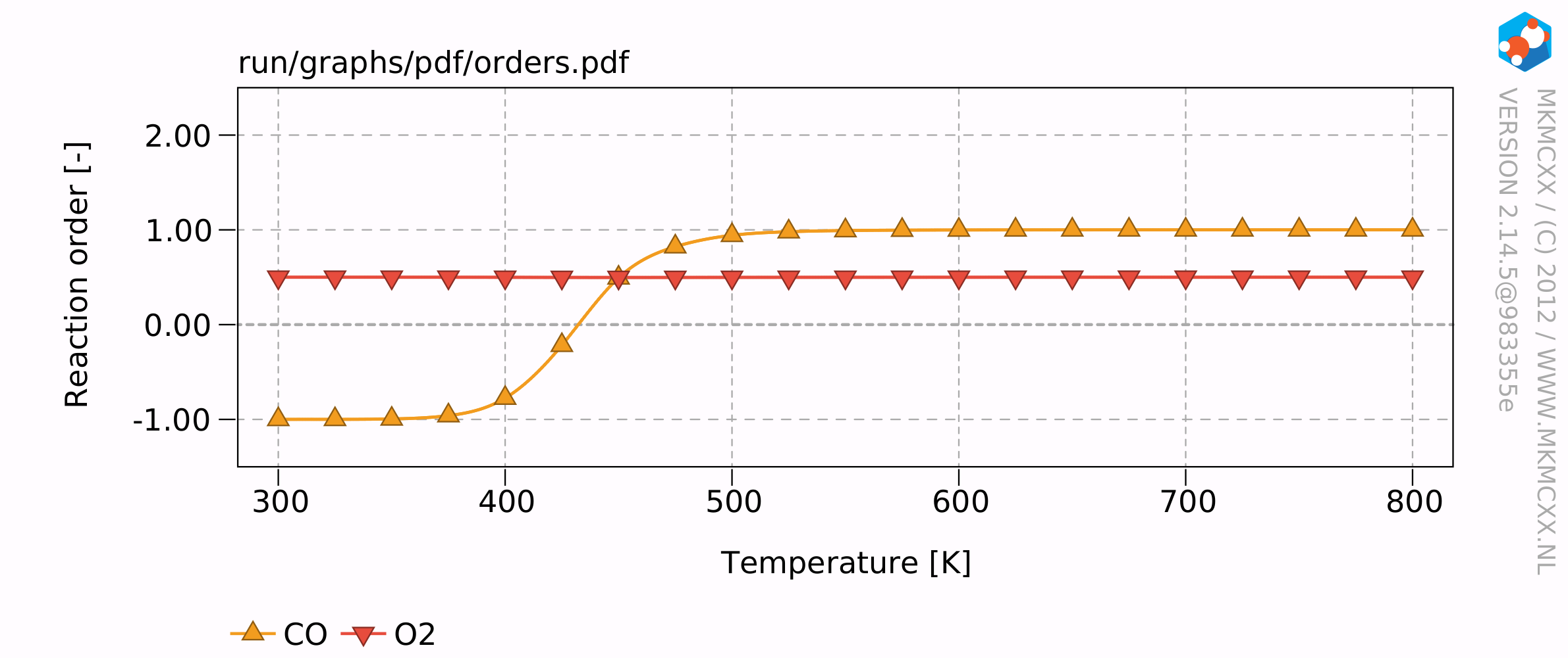
The results of this example calculation show that the reaction rate reaches a maximum around 500 K. The reaction order for CO starts at -1 and increases to +1 at high temperatures and an empty surface. The reaction order for O2 remains at 0.5 throughout the temperature range. This means that when the partial pressure of O2 quadruples, that then the overall reaction rate would double.