Kinetic Monte Carlo

In this tutorial we will walk you through a Kinetic Monte Carlo (KMC) calculation with the program Zacros, using the GUI. The GUI will generate a pyZacros script that can be run via AMSjobs, just like other runscripts. And with some python experience it should be no problem to extend this script for more advanced tasks.

See also

• AMSkinetics-GUI manual

• pyZacros manual

• Zacros documentation in $AMSHOME/scripting/scm/pyzacros/doc/ZacrosManual.pdf

We will setup the Ziff-Gulari-Barshad model. This will be the same model as in the tutorial on the Zacros website and in the pyZacros tutorial, where more info on the model can be found.

Tip

If you only want to run the simulation without setting it up, download zacros_tutorial.kin. To open it, first open AMSkinetics (SCM → Kinetics), select File → Open and browse to the file.

Step 1: Specify general settings

We will start the AMSkinetics module to create our setup. Depending on your license, you might not need to switch to the Zacros program.

1. Start AMSjobs.

2. Click on SCM → Kinetics.

3. Switch to the Zacros program by clicking on the yellow arrow MKMcxx → Zacros.

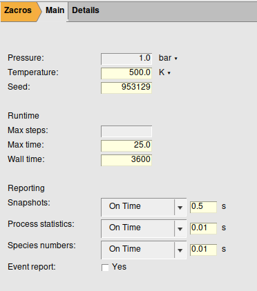
In the first step we will specify the general calculation settings. In AMSkinetics they are found on the right panel. The general settings include the conditions of the system, such as the temperature and pressure. A random seed can be specified, such that multiple runs will produce the same results. Multiple stopping criteria can be specified, either based on the calculation time or steps, or the real “wall” time. Finally there are the sampling setting: snapshots, process statistics and species numbers. Those can be individually set per event (most useful for test runs) or time step.

All the general settings in the GUI are equivalent to the Zacros input options in simulation_input.dat. These will be generated as pyZacros Settings object in the runscript.

We will use the following settings in our setup:

Set 500.0 K as the Temperature.

Set 1.0 bar as the Pressure.

Set 953129 as the Seed.

We leave the Max steps empty, this will use maximum possible.

Set 25.0 for the Max time.

Set 3600 for the Wall time.

We will use On Time for all sampling settings.

Set 0.5 for the Snapshots.

Set 0.01 for the Process statistics.

Set 0.01 for the Species numbers.

Step 2: Specify the species

The gas and surface species can be added on the left panel. There you can switch between the different input settings via the tabs. In this step we will start with the Gas species.

With the you can add new gas species. It is also possible to paste preformatted data from a spreadsheet, instead of entering the values by hand. Fields can be left empty, a default value of 0.0 eV for Gas energy or 0.0 as initial Molar fraction will be used.

We will use the following gas species in our setup:

Add a new CO species with 0.45 for the Molar fraction.

Add a new O2 species with 0.55 for the Molar fraction.

Add a new CO2 species with -2.337 eV for the Gas energy.

Next, we will add the surface species on the Surface species tab. By default, there is always the empty site *. The surface species names conventionally have * characters at the end to denote the denticity of the species. AMSkinetics will fill in the denticity correctly if the surface species names follow this convention.

Add a new CO* species. It is a monodentate species.

Add a new O* species. It is a monodentate species.

In later steps the gas and surface species will be used to setup Clusters and Reactions. It is still possible to modify or add new species after setting up Clusters and Reactions. In Zacros the species are part of the simulation_input.dat file and are handled the same. They will be generated as pyZacros Species in the runscript. In pyZacros the Molar fractions are part of the Settings object, to aid more advanced scripting.

Step 3: Specify the lattice structure

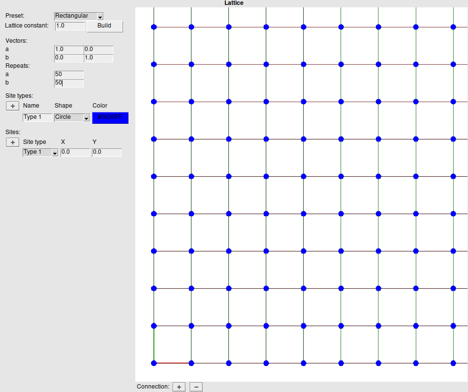
The lattice structure is found on the middle panel. There on the left there are tools to build the lattice. You can use a Preset from the list, specify the Lattice constant and click Build to create a new lattice. This will delete any created Clusters and Reactions, as those depend on the possibly deleted sites. The Presets are the default lattices that can be specified in Zacros. However, these can be further modified and will be passed on as a Unit-Cell-Defined Periodic Lattice.

The lattice Vectors can have custom values or can be set by the previously mentioned Preset. The Repeats can be modified at any point, so are not necessary when using the Preset. It can be kept at 1 repeat if a complete custom lattice is desired.

Finally it is possible to create new Site types and add new Sites.

On the right is an interactive lattice display.

Scroll to zoom.

Left-click drag to pan the view.

Left-click a site to select or deselect the site.

Left-click on an empty spot to deselect all sites.

Right-click a site to choose do delete the site.

Right-click an empty spot to choose to add a new site.

Right-click drag a site to move the site.

Below the lattice display you can add or remove connections between selected sites.

We will build the lattice using these steps:

Select the Rectangular preset

Specify a Lattice constant of 1.0

Click Build

Set the Repeats for both lattice vectors to 50

In Zacros the lattice settings are in the lattice_input.dat. They will be generated as pyZacros Lattice in the runscript.

Step 4: Specify the energetics model: Clusters

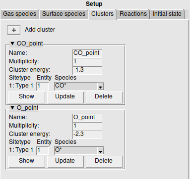
Clusters are found on the left panel under the Clusters tab. Clusters are represented as a graph. We can define these by selecting one or more connected sites from the lattice. This makes sure the graph actually exists in the defined lattice, and immediately gives a good visualization of the graph. After selecting the pattern you can click the to add a new cluster.

The Multiplicity counts the amount of times the representation is found on the lattice. It will divide the Cluster energy, but can be kept at 1 if the cluster energy is already normalized. Finally the Species can be assigned to the selected sites. Multidentate species should have the same Entity number on each bound site. When saving the final setup, the GUI will check if this is consistent. You can Show the cluster on the lattice, which selects and labels the sites. The sites closest to the origin are used to show the cluster representation. You can Update the cluster to change the graph to the new selection, or Delete to remove the cluster.

We will add two clusters, for CO* and O*:

Select a site on the lattice.

Add a new cluster with .

Name it CO_point.

Set the Cluster energy to -1.3 eV.

Select CO* as the Species.

Add a new cluster with

Name it O_point.

Set the Cluster energy to -2.3 eV.

Select O* as the Species.

In Zacros the cluster settings are in the energetics_input.dat file. They will be generated as pyZacros Clusters.

Step 5: Specify the reaction mechanism: Reactions

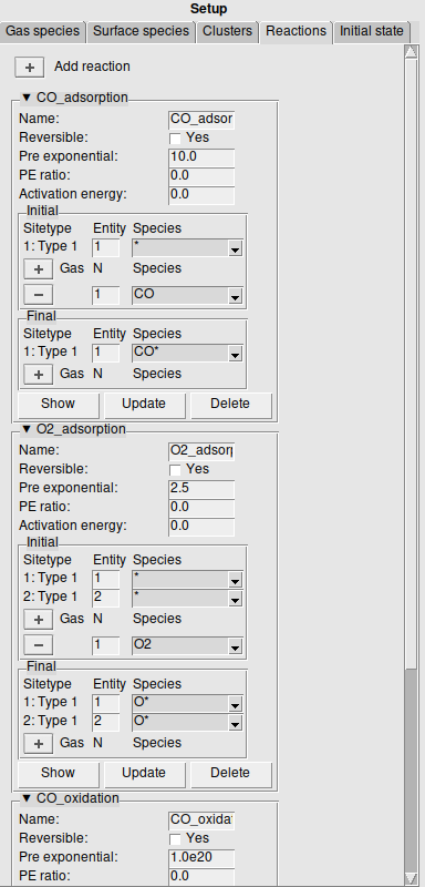
Reactions are found on the left panel under the Reactions tab. Just like clusters, reactions are represented as a graph, and are defined via the same method. Each site now represents the initial and final state of an elementary event.

The Reversible checkbox indicates that the reaction is reversible. The Pre exponential specifies the pre-exponential for the forward reaction in the Arrhenius formula. For reversible reactions the PE ratio specifies the ratio between the forward and reverse pre-exponentials. The Activation energy specifies the activation energy at the zero coverage limit for the forward reaction.

For each site the Initial and Final species can be specified. Again, like for the clusters, the Entity number should be the same for multidentate species. Additional Gas species can be specified for each side of the reaction. The Show, Update, and Delete work the same as for the clusters.

We will add 3 reactions; two adsorption reactions and the oxidation reaction:

Select a single site on the lattice.

Add a new reaction with .

Name it CO_adsorption.

Set Reversible to Off.

Set the Pre exponential to 10.0.

For the Initial side keep the * empty site.

Add a Gas species and set it to CO.

For the Final side choose the CO* species.

Select 2 connected sites on the lattice.

Add a new reaction with .

Name it O2_adsorption.

Set Reversible to Off.

Set the Pre exponential to 2.5.

For the Initial side keep both * empty sites.

Add a Gas species and set it to O2.

For the Final side set both sites to the O* species.

Select 2 connected sites on the lattice.

Add a new reaction with .

Name it CO_oxidation.

Set Reversible to Off.

Set the Pre exponential to 1.0e20.

For the Initial side choose a CO* species and a O* species.

For the Final side keep both * empty sites.

Add a Gas species and set it to CO2.

In Zacros the reaction mechanism settings are in the mechanism_input.dat file. They will be generated as pyZacros ElementaryReaction.

Step 6: Run and analyze the results

The Initial state tab on the left panel is not used in this tutorial. It can be used to either randomly or specifically populate sites with surface species for the initial state.

We will now save and run the setup. This will generate a file ending with .kin which is used to store the GUI setup, which can be opened again later by AMSkinetics. This is analogous to the .ams files for AMSinput. The runscript is as usual saved in a .run file, and contains the full pyZacros script.

Use File → Save to save the setup as ZGB.

Use File → Run to run the calculation.

All the files that pyZacros generates and the output of Zacros will end up inside the .results directory. If the AMSkinetics module is still open, it will now ask to analyze the results. You can also analyze the results via View → Results.

Answer Yes to analyze the results.

This will bring up Zacros-post, a program for analyzing Zacros results. If you do not have Zacros-post installed, it will prompt you to install it. Zacros-post can also be installed or uninstalled using the SCM package manager (SCM → Packages).

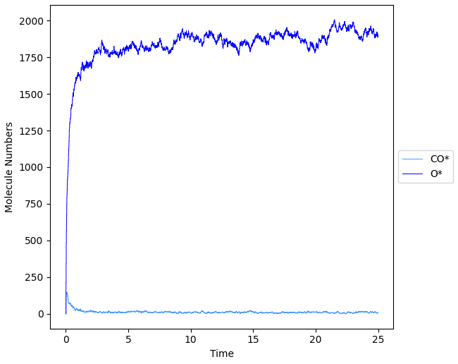
In Zacros-post, you can for example select Plot → Species Numbers to see the surface species as a function of time

Other examples

• Download zacros_reversible.kin for an example with reversible reactions, based on A Simple KMC simulation from zacros.org