Young’s modulus, yield point, Poisson’s ratio
Details on the calculation of atomic stresses can be found in the ReaxFF manual .
Note
The calculations are computationally demanding. For optimal performance, a parallel execution on a compute cluster is advised. This can best be done by using the remote job management of the GUI
The simulation may take several days.
Tip
For crystals you can also calculate the Young modulus and Poisson ratio with the elastic tensor.
Overview
This advanced ReaxFF tutorial is based on Radue, Jensen, Gowtham, Klimek-McDonald, King and Odegard, J. Polym. Sci. B, 56, 255-264 (2018). It will demonstrate how to calculate stress-strain curves of an epoxy polymer.
Contents:
Setting up a strain rate
Calculate the atomic stresses
Results: stress-strain curves, Young’s modulus, yield points…
Tip
The molecular structure used in this tutorial was kindly provided by Matthew S. Radue. Other highly cross linked epoxy polymers can effectively be created with a novel bond boost acceleration method (see tutorial).
Setting up
The polymer used in this tutorial is referred to as Tetra(-epoxy) in Ref. 1 since it was build from the tetrafunctional resin epoxy TGDDM (tetra-glycidyl-4,4 0 - diaminodiphenylmethane, Araldite MY 721) and DETDA as hardener. The following cross linking reaction was used to create the polymer structure:

Start by importing the polymer structure into AMSinput
here to download the .xyz file tetra_epoxy.xyzBefore setting up the strain rate, start with the general molecular dynamics settings. Begin by selecting a force field
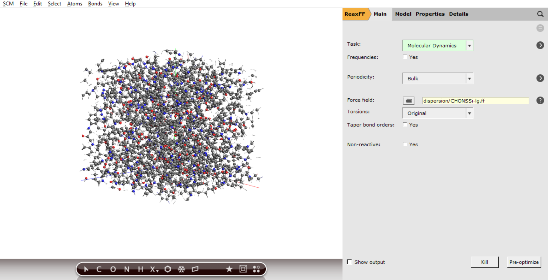
 next to Molecular Dynamics
2000000 as Number of steps (500 ps)2000 as Sample frequency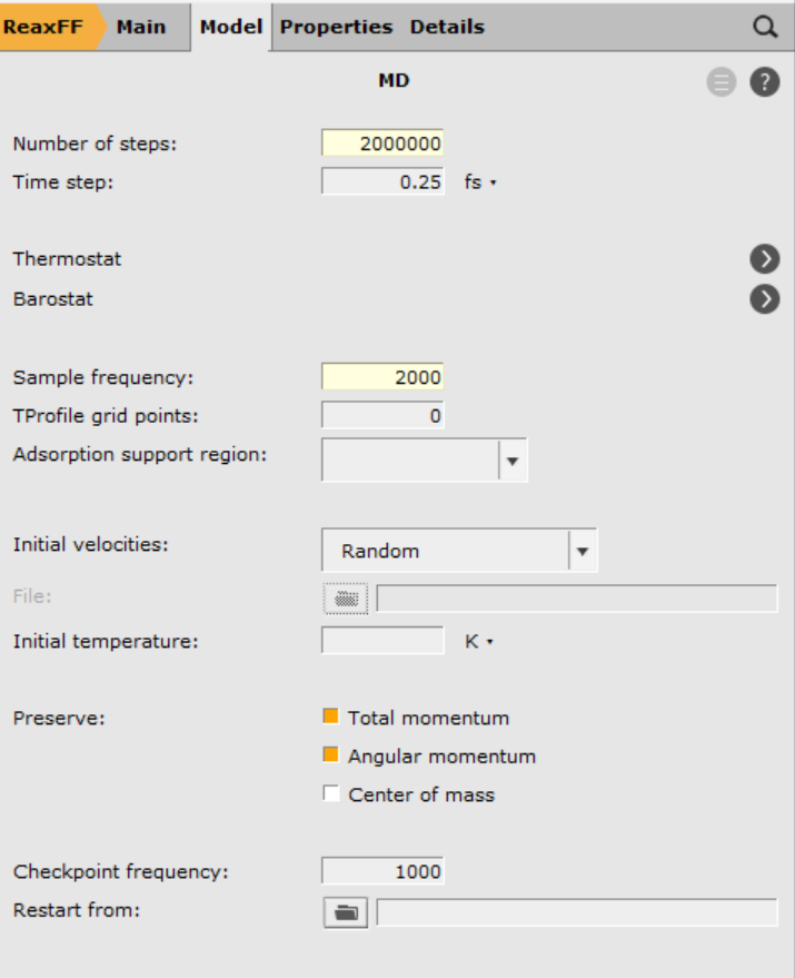
Next we set up the thermo- and barostat
next to Thermostat
300.15 K and the Damping constant to 100 fs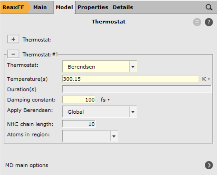 next to MD main options next to Barostat
101000 Pa and the Damping constant to 1500 fs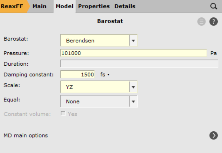
Note
We are applying uni-axial strain, i.e. alongside one lattice vector, and apply the barostat only in the lateral directions. This will allow us to account for Poisson contractions.
Setting up the strain rate
The publication Ref. 1 put a linear strain of 20% over the course of 1 ns. Since we are simulating only 500 ps, for the sake of computational efficiency, the total strain reduces to 10%.
The straightforward way to defining this strain is by defining the strain type to be linear, followed by the final length of the vector at the end of the straining.
Let’s first find and note the length of the a-lattice vector.
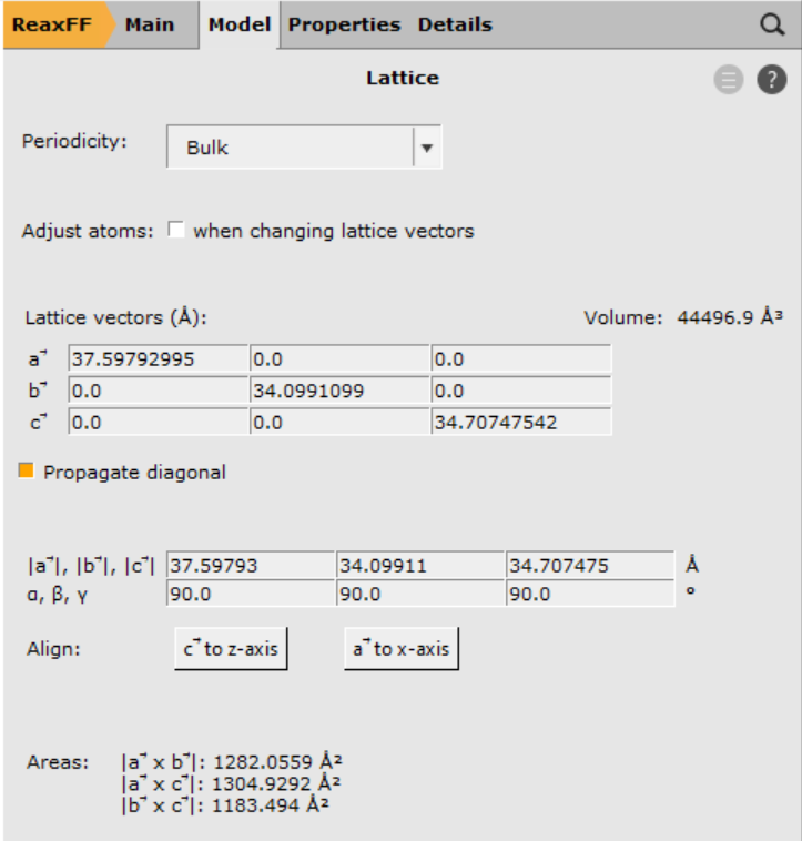
The length of the a-lattice vector a (\(\mid\vec{a}\mid\)) is found to be 37.59793 Å. The endpoint, after stretching it 10%, will then be 41.36 Å. To define this strain, change to the MD deformation panel
2000000 as the final step41.36, 0, 0 as the final lengths of the lattice vectors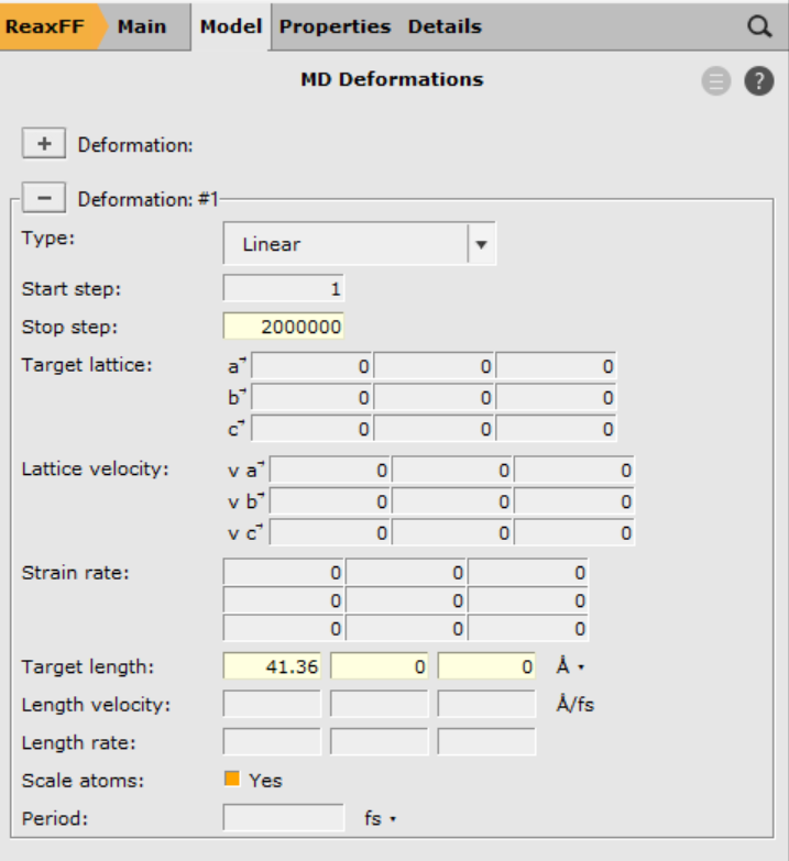
Tip
Putting a 0 as final length tells the program to ignore that particular lattice vector. You can learn about the meaning of each input field by hovering your mouse pointer over it.
Save the input files with a suitable name, e.g. tetra_strain_a, and run the calculation.
On 16 cores, it will typically take a bit less than 1 day to compute the trajectory depending on your hardware.
Results
The results can be analyzed either using the AMSMovie GUI module or via a python scripting.
Important
In order to get statistically and physically meaningful results, it’s advised to average the mechanical properties, both over different starting structures as well as all three unaxial strain directions. To obtain quality results as in Ref. 1, an averaging over 5 different polymer structures using 3 strains each (15 trajectories) is required.
Your results may look different from the plots below.
Once the calculation is finished, open the results with AMSMovie:
Let’s remove the Energy v.s. time graph, which is not useful for our purposes here:
The Young’s modulus can be computed via a linear regression on the Stress-Strain curve. AMSMovie already has a preset for computing the Young’s modulus:
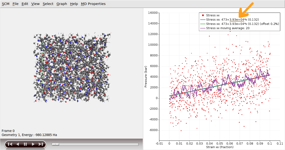
The graph displays the Stress-Strain data, as well as a smoothed version using a moving average and linear regression lines. The legend presents the coefficients of the linear regression and the corresponding r2 value, enclosed in parentheses.
The Young modulus is the slope of the Stress-Strain linear regression, which in this case is 3.39 * 10^4 bar (or 3.39 GPa).
Note that by this linear regression is performed using the whole strain range (from 0 to 0.1). Following Ref. 1, we will now show how to compute the Young modulus in a smaller strain regime (e.g. only considering the strain range from 0 to 0.03).
0.03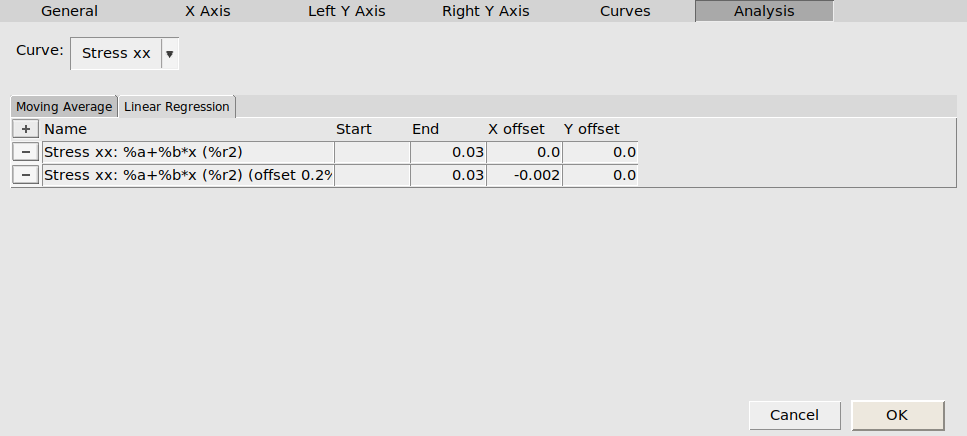
In the plot, you can see that the value of the Young modulus (i.e. the slope coefficient of the linear regression) has changed, since now it’s computing the linear regression only using the values in the 0 to 0.03 strain range. The value of the Young modulus in the 0-0.03 strain range is 5.4 GPa.
In principle, one could calculate the Yield Point using the method outlined in Ref. 1, which involves finding the intersection point between a moving average and the 0.2% offset regression line. However, one would need more statistics / data to get any meaningful result (for example, in Ref. 1, an averaging over 5 different polymer structures using 3 strains each was used)
Tip
In the Analysis Graph options (Menu: Graph → Analysis) you can change the window for the moving average.
Finally, we can compute the Poisson’s ratio (obtained from a linear regression of the transverse strains):
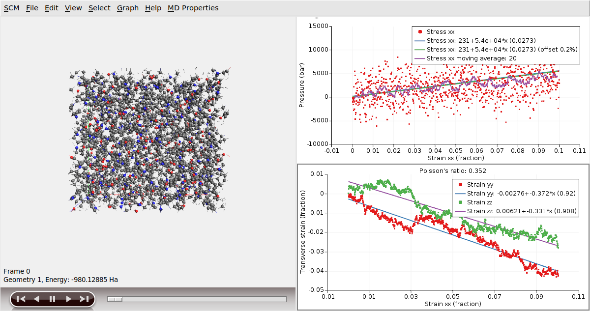
Since the system is amorphous, the Poisson’s ratio is the average of the two slopes (0.352 in this case).
The stress-strain curves can be extracted from the binary results file with the help of a Python script using the PLAMS library.
The script called stress_strain_curve.py can be run from the command line:
$AMSBIN/amspython stress_strain_curve.py tetra_strain_a
Be sure to match the job name correctly.
The stress-strain curve is written to a file called stress-strain-curve.csv:
strain_x, strain_y, strain_z, stress_xx, stress_yy, stress_zz
0.0001 -0.0012 0.0016 -0.0126 0.0107 -0.0142
0.0002 0.0003 0.0025 ...
It can be plotted with any graph plotting software, e.g. gnuplot or qtiplot. You can also use the script young_yield_poisson.py. Call it with $AMSBIN/amspython young_yield_poisson.py stress-strain-curve.csv. The python script creates the plots shown below and calculates the Young’s modulus, yield point, and Poisson’s ratio.
The following example shows how to obtain the mechanical properties from stress-strain plot for an uniaxial strain in x-direction (column 4 plotted vs column 1):
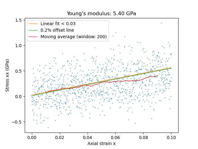
A Young’s modulus of 5.4 GPa was calculated from the slope of a linear regression to the small strain regime (< 0.03) (orange line).
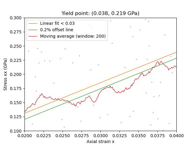
The yield point is then found as the intersection between
the moving average line (200 points for smoothing), red, and
a 0.2% offset line (shifted by 0.002 along x) of the linear fit, green.
Poisson’s ratio is obtained from the ratio of transverse and uniaxial strains, i.e. plotting column #2 and #3 against column #1 (the system was strained in the x-direction)
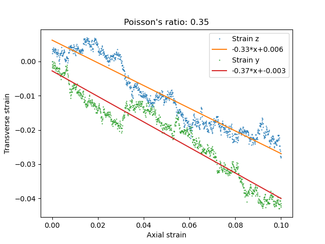
Since the system is amorphous, Poisson’s ratio is the average of the two values.
Literature: