Combustion simulation (ReaxFF)
This tutorial will show you how to:
create a simple mixture (methane and oxygen)
set up a quick combustion reaction (using ReaxFF)
burn it: perform the actual ReaxFF simulation
visualize what is happening during and after the simulation
Step 1: Start the GUI
 →
→ 
Step 2: Create a methane / oxygen mixture
Next we will make the methane - oxygen mixture. For full combustion we need at least 2 oxygen molecules for each methane molecule. So we will use 50 methane molecules and 125 oxygen molecules.
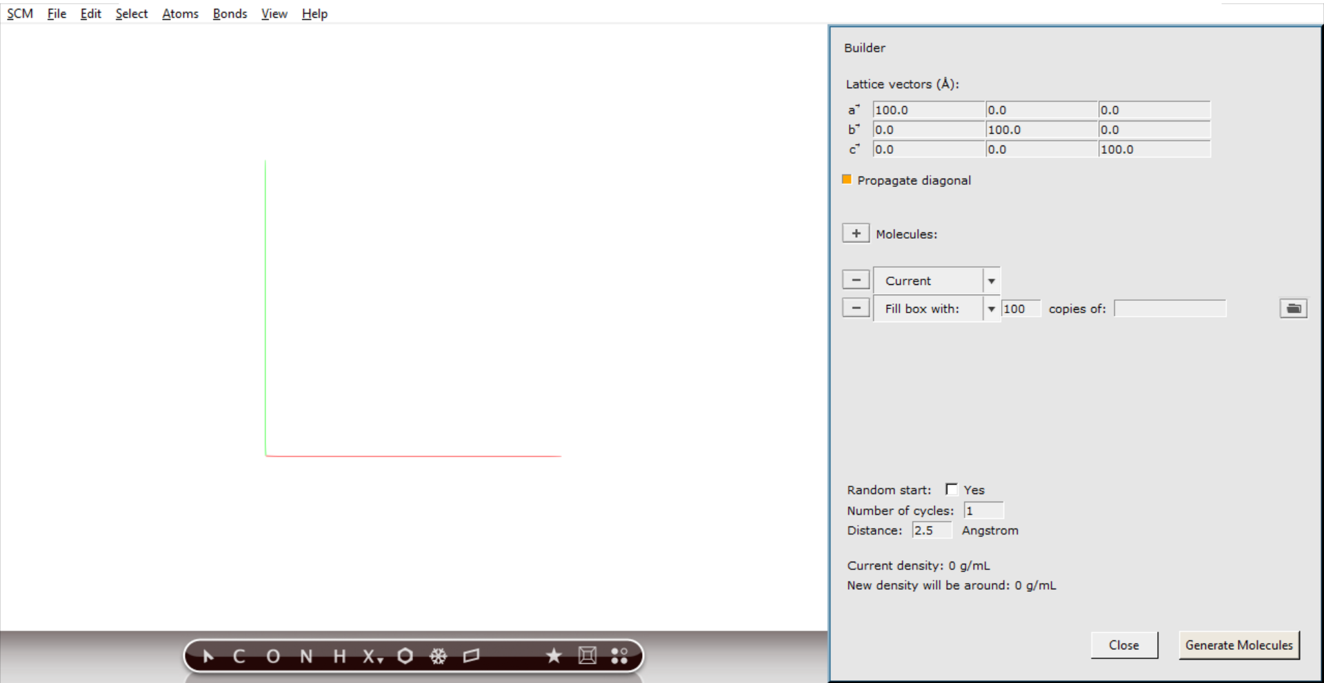
The Builder allows you to build your system, and set some things like the cell vectors that define the computation cell.
You can use the Builder to add many molecules, randomly distributed. In the list of molecules to be added the current molecule is already present. If you have any molecules already, the new molecules will be added. Right now we have no molecules yet, so we can remove that entry.
19 on the diagonal to change the box to a cube of 19.0 Angstrom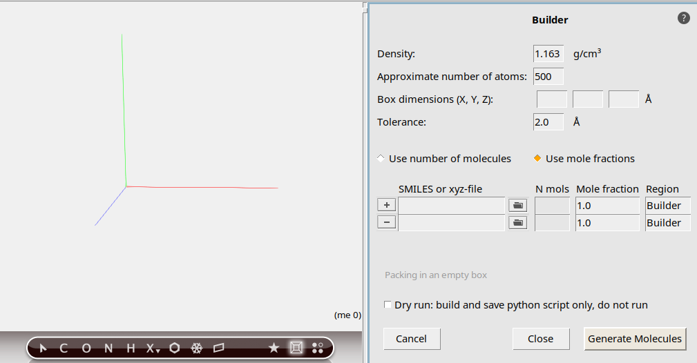
met to search for methane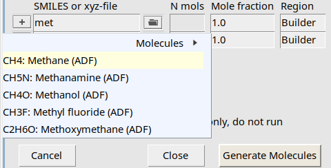
As you can see, a search box appears to find your molecule, very similar to the search box in the panel bar.
50o to search for O2125 copiesYou now have specified how the builder should build your system: 50 methane molecules with 125 oxygen molecules added.
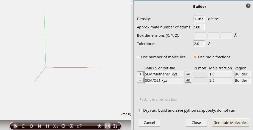
At the bottom of the Builder panel you can see that the current density is zero. The new density, after adding methane and oxygen, will be around 1 g/mL, which is obviously very high for this mixture. In this tutorial, we simply want things to happen fast, so this high density is acceptable.
Next we will actually generate the molecules:
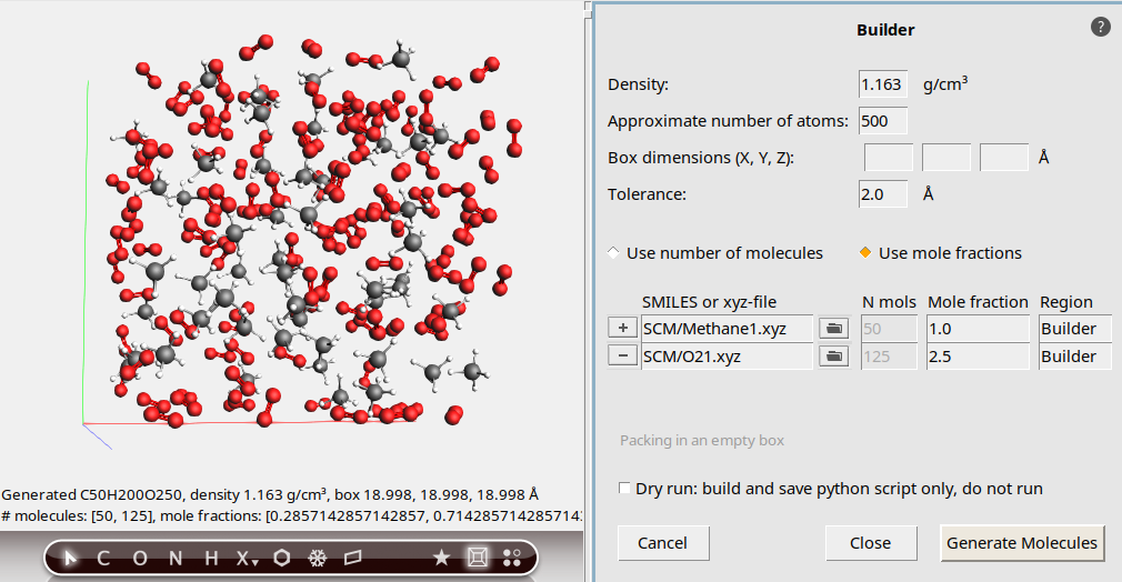
The molecules are generated at random positions and orientations, with constraint that all atoms (between different molecules) are at least the specified distance (2.5 Angstrom) apart.
The system looks good, we can now close the Builder:
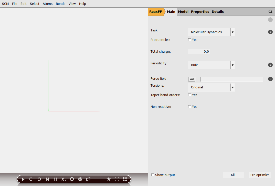
Step 3: Prepare for burning: set up the simulation
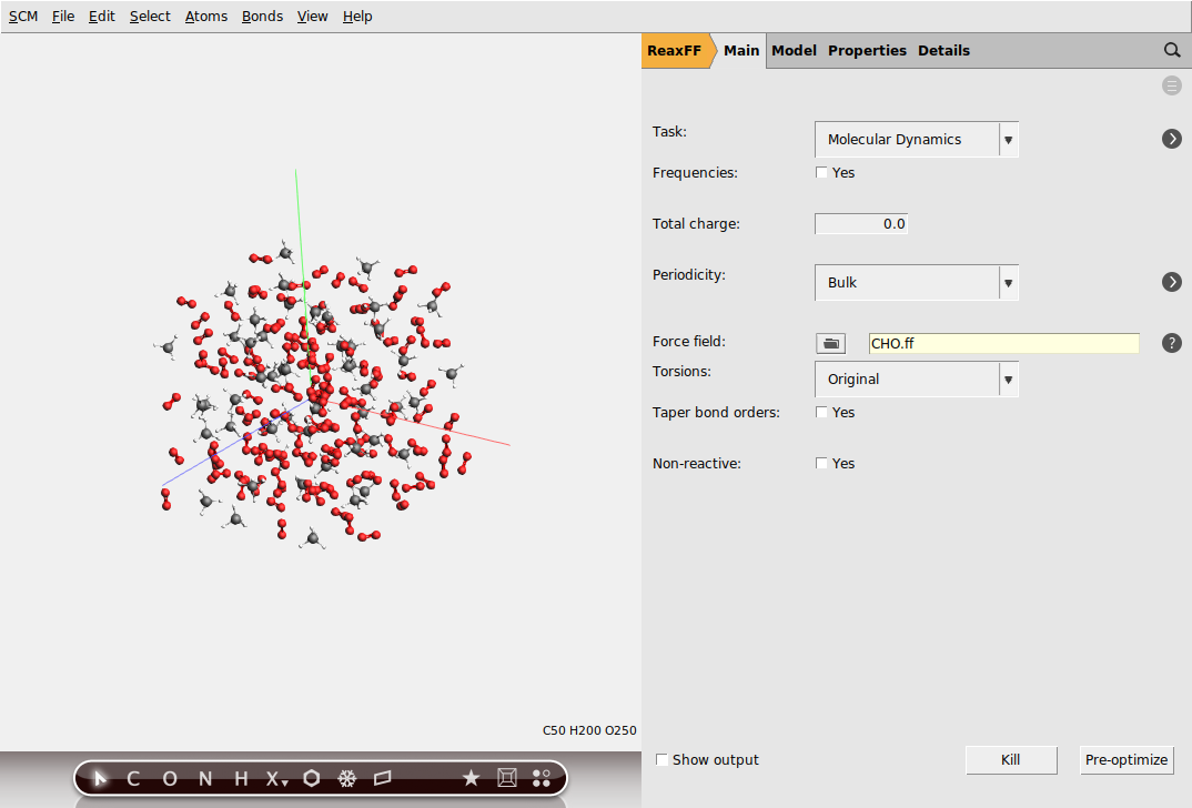
The next step is to set up the details of the simulation.
Note
For this tutorial we will perform an MD simulation at very high temperature and density in order to make reactions happen quickly. This is meant to be a quick demonstration of functionality rather than a realistic representation of this system.
 on the right side of the Force field line
A new window should appear describing what force fields are available, including a short description and references. For this particular example we will use the CHO force field for hydrocarbon oxidation.
Change to the MD settings panel:
 next to Molecular Dynamics
30000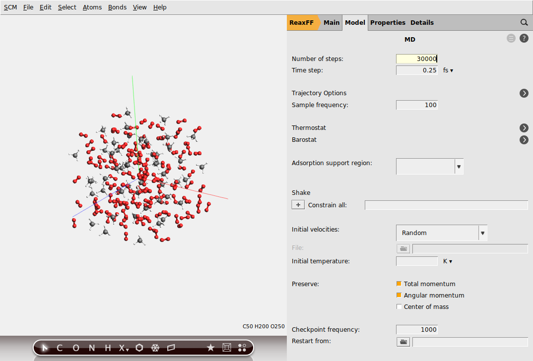
Note
We will be using the Nose-Hoover thermostat which yields better overall sampling results in general. The Nose-Hoover damping constant is dependent on the system size because ideally it should match the period of the internal oscillations of the system. In the present case we stick to the default value of 100 fs but one might want to test different values in a realistic setup.
To setup a Nose-Hoover thermostat with a damping constant of 100 fs, change to the Thermostat panel:
next to Thermostat
3500 K and a Damping constant of 100 fs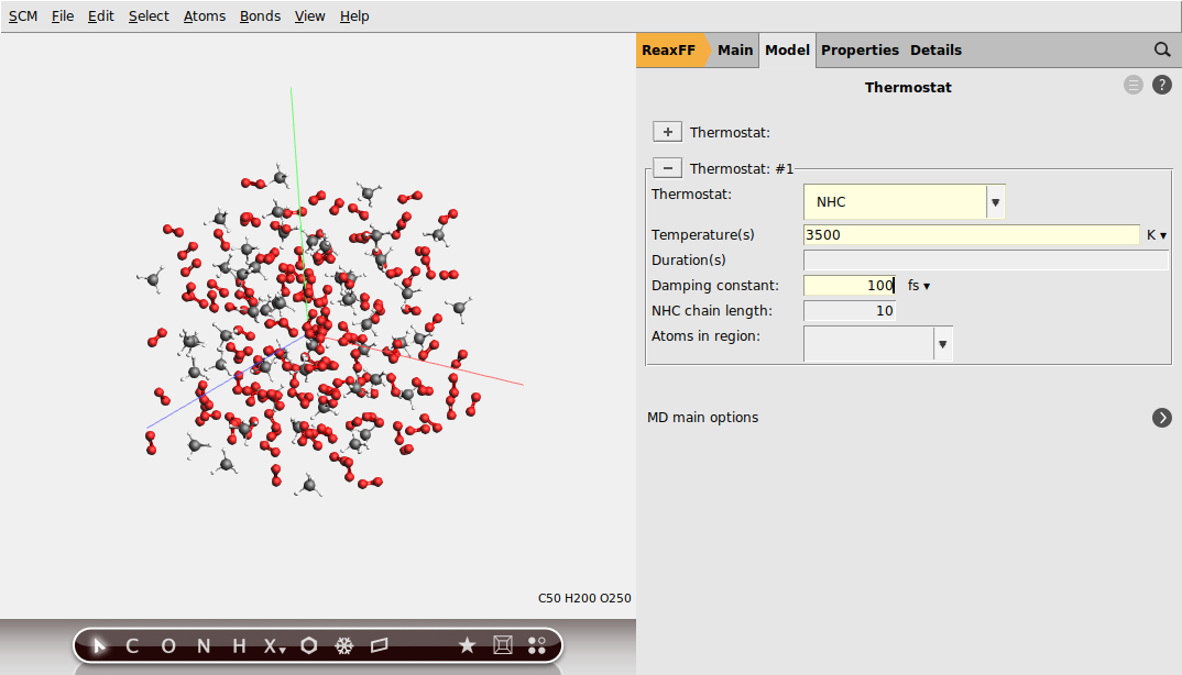
Step 4: Burn it: run the simulation
Now we will run your set-up:
MethaneNote
Running this calculation takes approximately 10 minutes. You can do the following steps while the job is running.
AMSjobs should come to the foreground, and your job should be visible at the top. On the right side you can see that the job is running (this is indicated by the gear-icon). When running, in the AMSjobs window the progress of your simulation is showing (from the logfile). When you click on the progress lines the logfile will open in its own window:
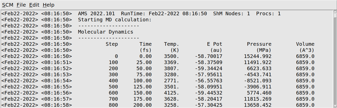
As you can see in the logfile, the simulation is running.
To see more details, we now will use AMSmovie. Note that you can do this while the simulation is still running!
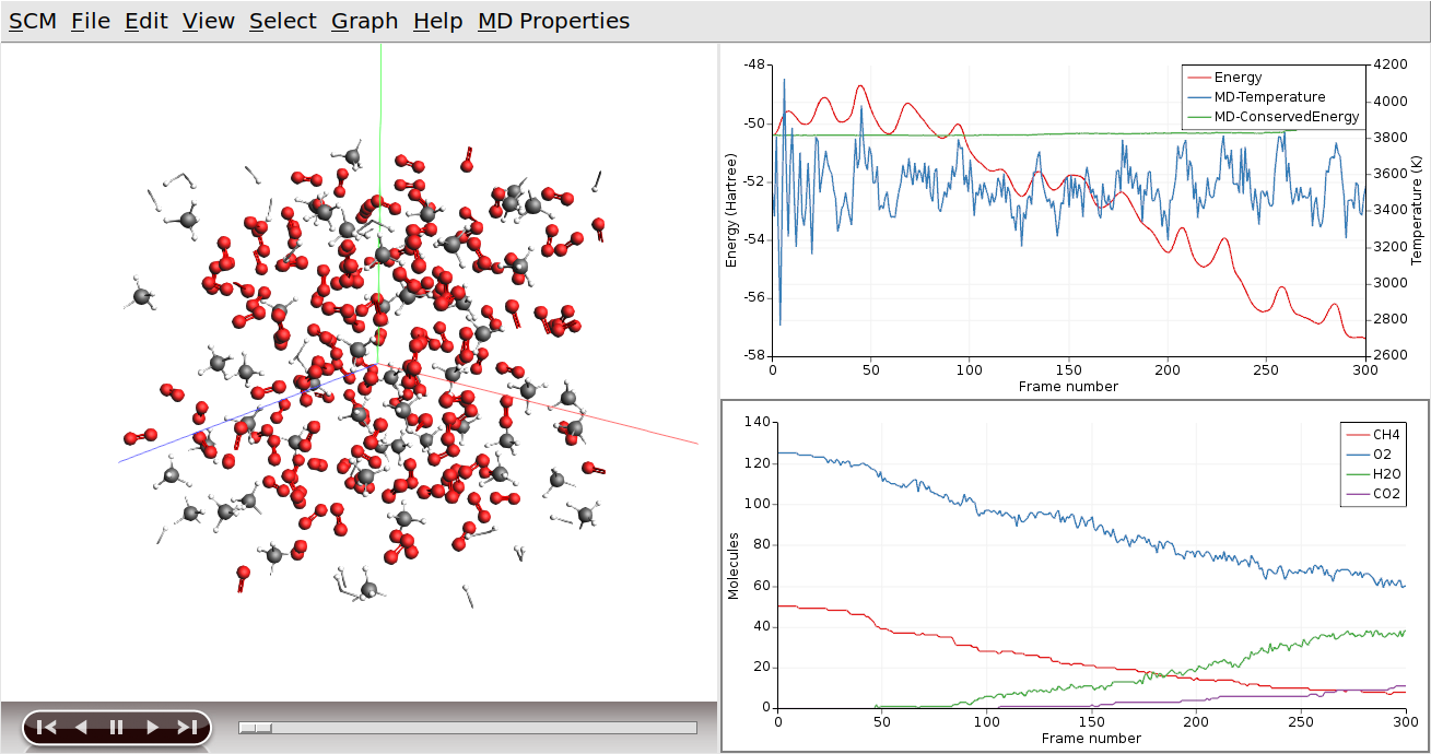
AMSmovie will show you the trajectory of your system. Note that it will automatically read new data as soon as it becomes available.
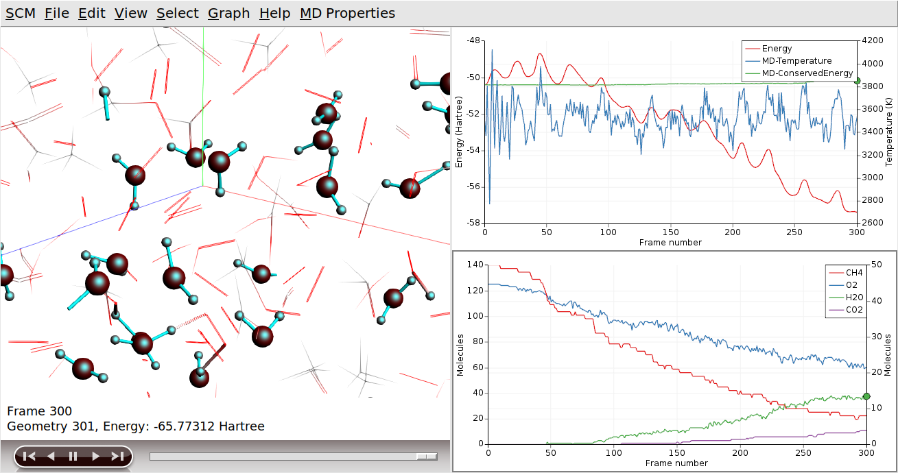
It can also show graphs of the properties that ReaxFF calculates:
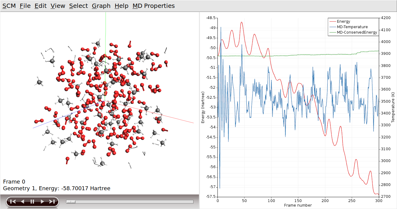
You can go to a particular point in the simulation using the slider below the window showing your system, or you can click somewhere on one of the curves plotted. You can also use the arrow keys (left and right) to move through the simulation.
Tip
Click on the temperature curve to move around in the movie. Jump to the end of the movie to follow the progress
As ReaxFF is a reactive force field, reactions may take place. In this particular example the methane should react with the oxygen, eventually producing H2O and CO2.
You can make graphs that show how many of the different molecule types are present. The following instructions often work, but it depends on what molecules are present in your simulation. You might try this step again after waiting some time. Remember that we only requested 30000 iterations, so you might consider rerunning the tutorial with an increased amount of steps. Especially the production of H2O and CO2 take some time.
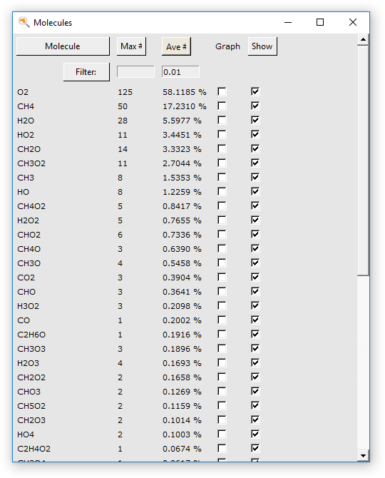
In the dialog window that appears all molecules that occur in the calculation are shown (up to the moment the dialog is created). By clicking at the top in the dialog you can sort the molecules by name, occurrence in the last frame, or average occurrence.
Warning
The information shown in the molecules dialog does NOT automatically refresh for a running calculation.
To refresh: close the dialog, and use the MD Properties → Molecules… command again.
The first column of check boxes allow you to select for which molecules to show a graph of their occurrence (the number of molecules of the selected type, per time step).
The second column allows you to show or hide that particular molecule type. This can be convenient to hide the original molecules for example, so you can easily see what is happening.
The two text entry fields at the top are thresholds used to filter the number of species shown. In this particular tutorial they are not needed, all molecule types are visible. But if you are dealing with a system with many thousands of species the dialog would otherwise no longer be usable. Obviously you can adjust the filter values to your needs, and reapply them by clicking the Filter button.
Tip
You can drag the legend in the plotting area around with the mouse
You can put one of the curves on a different axes if you wish:
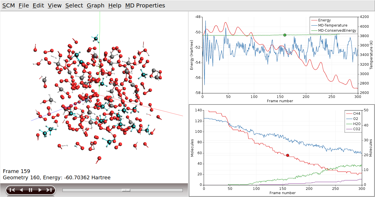
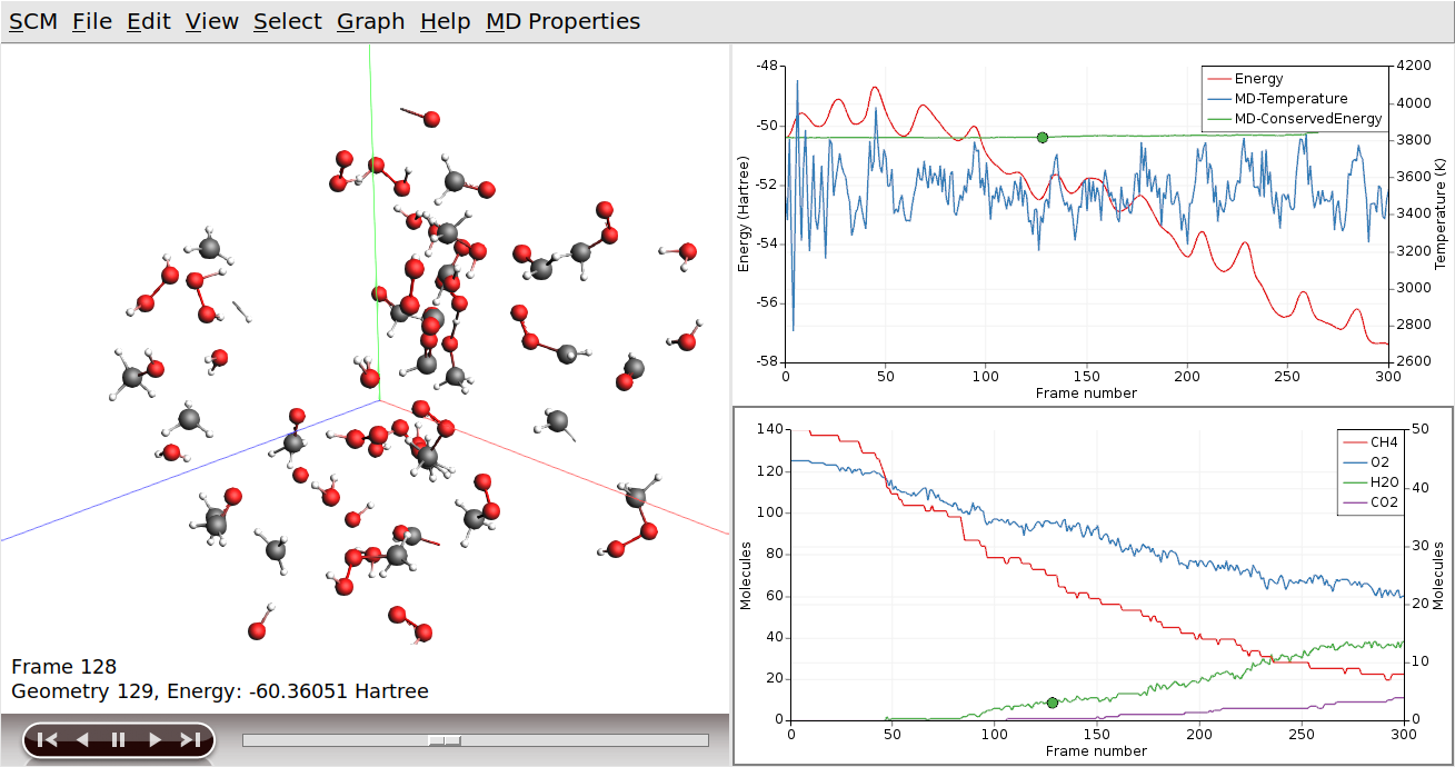
Clicking on the curve also had two other effects (besides making it the active curve): you jumped to the iteration in the movie corresponding to the point where you clicked, and the molecules that belonged to that curve are selected.
Flying to the selection also makes it easier to spot them:
To see the CO2 molecules clearly, we will switch everything but the CO2 molecules to wireframe.
Tip
The visualization style in the View → Molecule command applies to the selection only, if any
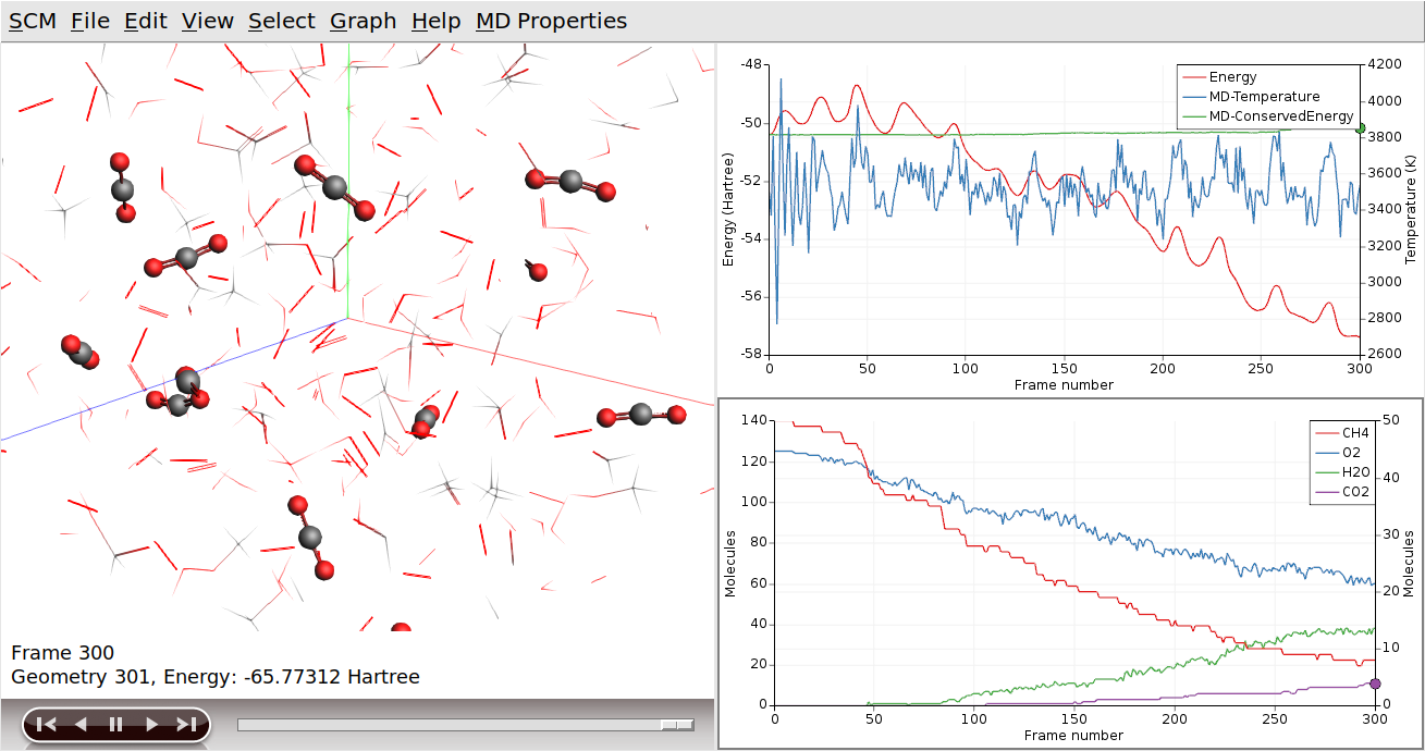
When you now go forward or backwards in time, it is easier to see how the reactions actually take place. Note that the atoms remain selected, even if they are no longer part of a CO2 molecule. In a similar way you can focus on H2O produced:
Another tool to see what is going on is hiding molecule that are not of interest. In this example, let’s hide CH4 and O2:
There is another tool to focus on a region of interest, by showing only some selected part:
