2. General Output
The output of an ACErxn run consists of the created reaction network, as well as runtime information on how the network was obtained. All output described below can be generated by running the file cyclohexenone.run in the folder $AMSHOME/examples/acerxn/cyclohexenone.
2.1. The ACErxn Network
The main output of an ACErxn run is the created reaction network. This network is stored as a set of RKF files in the folder acerxn.results. The folder contains individual RKF files for all the intermediates, and all of them can be visualized by opening the ams.rkf file with AMSMovie (left side). The full network will also be visualized by AMSMovie (right side), but if the network is very large, this visualization will not be very helpful.
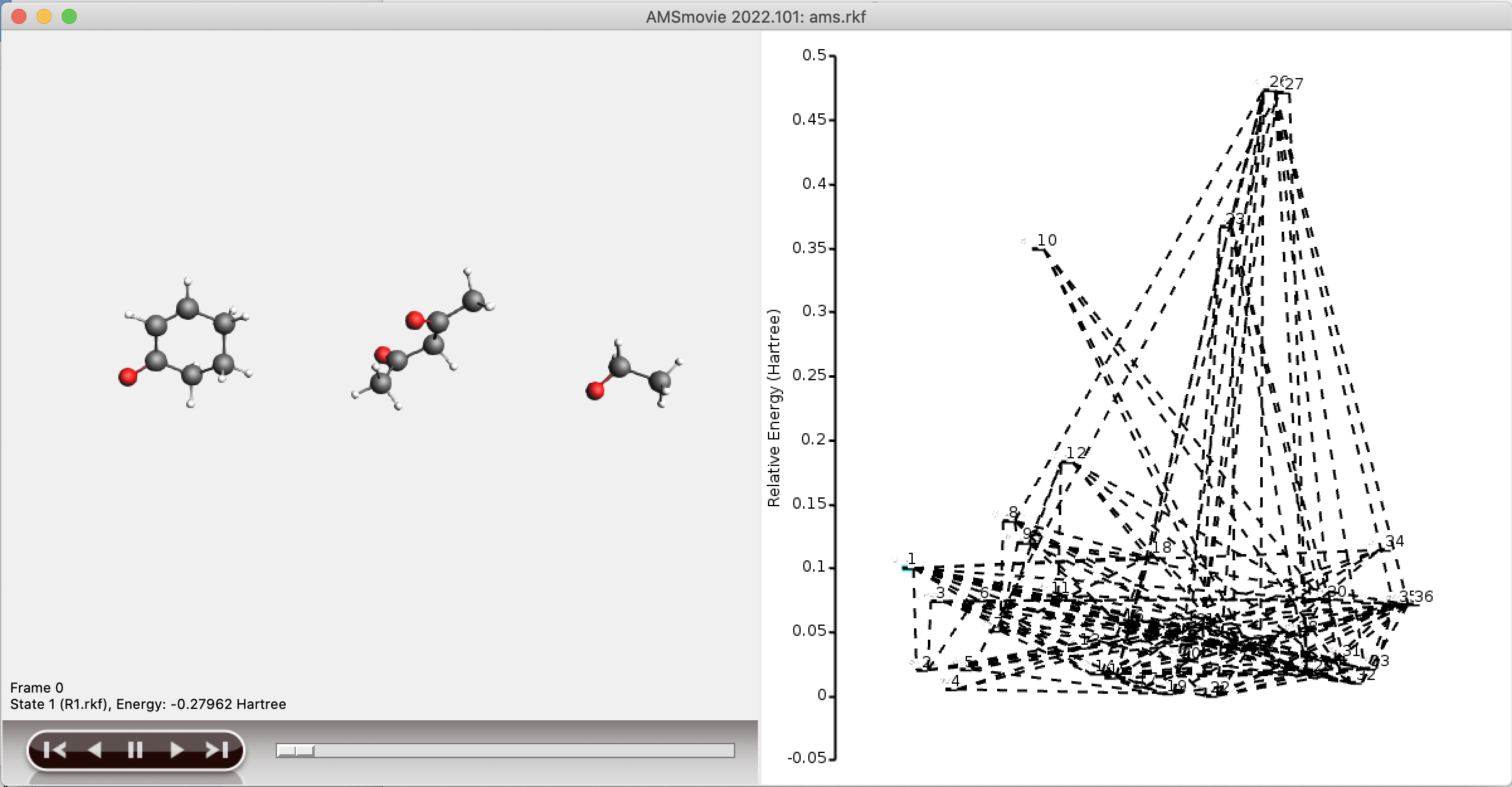
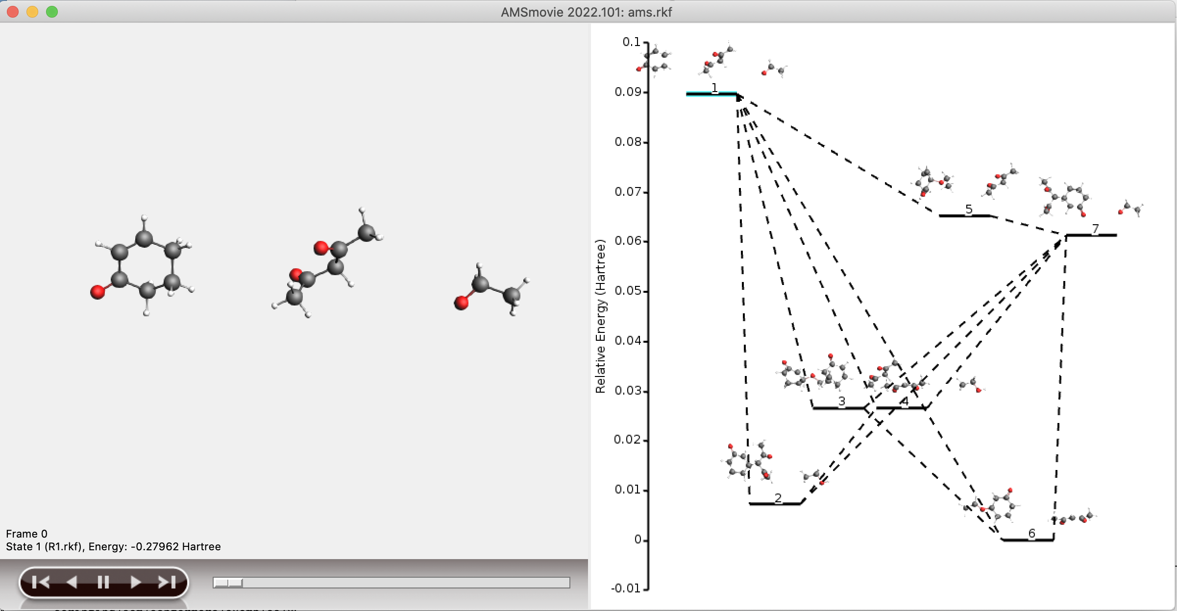
Since the full reaction network is often too large to conveniently visualize, a separate network is stored containing only the shortest paths from reactant to product. This subnetwork is stored in the folder plams_workdir/acerxn/shortest_paths. Generally, viewing the shortest paths in AMSMovie should yield a good overview of the structures involved in, and the potential energy profile of, the shortest paths.
Both reaction networks can be easily converted to a Python networkx graph using a simple Python script.
from matplotlib import pyplot as plt
import networkx
from scm.plams import init, finish
from scm.acerxn import ACErxnJob

# PLAMS
init()

# Read the networkx graph from the plams folder
job = ACErxnJob.load_external('plams_workdir/acerxn/acerxn.results',finalize=True)
graph = job.results.get_network().graph

# PLAMS
finish()

# Plot the network
networkx.draw( graph, with_labels=True, node_color='white', edgecolors='blue', font_weight='bold', node_size=4000 )
plt.show()
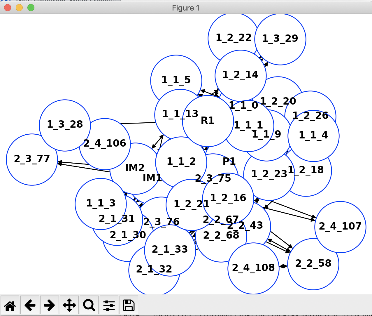
The conversion process will be useful for people familiar with the networkx Python module who can then manipulate the graph and the plot to their liking. Simply running the script above will result in the following plot of the full network.
2.2. Standard Output
At runtime, information about the progress of the different ACErxn steps is printed to standard output. The three steps of network creation are outlined below.
Intermediate generation: A set of intermediates is generated by enumeratively breaking and forming bonds in the reactant molecules.
Network creation: The intermediates are connected by elementary reactions, using filters based on the number of broken and formed bonds.
Network minimization: The most likely mechanisms from reactant to product are extracted, using shortest path algorithms.
2.2.1. Step 1
The output for the first step starts with input information on the reactant molecules, such as the indices of the active atoms, the active bonds, and any bonds that cannot be broken or formed throughout the intermediate generation process.
=================================
Step 1: Intermediate generation
=================================
===================
Settings enumerator
===================
Fragnum:  [1, 1, 2, 3, 4, 4, 4, 5, 6, 7, 8]
active_atoms:  [1, 4, 13, 14, 15, 19, 23, 27, 28, 29, 35]
all_bonds:  [(10, 9), (10, 8), (10, 7), (10, 6), (10, 5), (10, 4), (10, 3), (10, 2), (10, 1), (10, 0), (9, 8), (9, 7), (9, 6), (9, 5), (9, 4), (9, 3), (9, 2), (9, 1), (9, 0), (8, 7), (8, 6), (8, 5), (8, 4), (8, 3), (8, 2), (8, 1), (8, 0), (7, 6), (7, 5), (7, 4), (7, 3), (7, 2), (7, 1), (7, 0), (6, 5), (6, 4), (6, 3), (6, 2), (6, 1), (6, 0), (5, 4), (5, 3), (5, 2), (5, 1), (5, 0), (4, 3), (4, 2), (4, 1), (4, 0), (3, 2), (3, 1), (3, 0), (2, 1), (2, 0), (1, 0)]
forbidden and frozen:  [] [(1, 0)]
any atom-pair within fragment:  [(1, 0), (5, 4), (6, 4), (6, 5)]
active bonds:  [(1, 13), (1, 14), (1, 15), (1, 19), (1, 23), (1, 27), (1, 28), (1, 29), (1, 35), (4, 13), (4, 14), (4, 15), (4, 19), (4, 23), (4, 27), (4, 28), (4, 29), (4, 35), (13, 14), (13, 15), (13, 19), (13, 23), (13, 27), (13, 28), (13, 29), (13, 35), (14, 15), (14, 19), (14, 23), (14, 27), (14, 28), (14, 29), (14, 35), (15, 27), (15, 28), (15, 29), (15, 35), (19, 27), (19, 28), (19, 29), (19, 35), (23, 27), (23, 28), (23, 29), (23, 35), (27, 28), (27, 29), (27, 35), (28, 29), (28, 35), (29, 35)]
===================
This is then followed by information on the geometry optimization of the reactant molecules (three molecules in this example), first using a force field (MM) engine (default: UFF), and then the more accurate engine (QM) specified in the input. In the example below, the geometry optimizations of the three reactant molecules succeeded without incident.
---------------
Geometry optimization cycle 0
---------------
MM geometry optimizations (3)
timing MM optimization:  0.3057980537414551
QM geometry optimizations (3)
timing QM optimization:  0.35553479194641113
reactant energy -0.2796199566735772
Number of bond order matrices at start:  1
After optimization of the reactant geometries, the propagation process starts, where new intermediates are created by breaking and forming bonds in the reactant intermediate. Each propagation step results in a set of new bond matrices (BMs) representing the intermediates.
---------------------------------
Propagation count:  1
---------------------------------
BMs created this iteration:  23 ['1_1_0', '1_1_1', '1_1_2', '1_1_3', '1_1_4', '1_1_5', 'IM1', 'P1', '1_1_9', 'IM2', '1_1_12', '1_1_13', '1_2_14', '1_2_16', '1_2_18', '1_2_19', '1_2_20', '1_2_21', '1_2_22', '1_2_23', '1_2_26', '1_3_28', '1_3_29']
The names of the newly generated intermediates generally reflect the number of the propagation cycle, the index of the core it was generated on in a parallel process, and the index indicating when it was generated. The indices are non-consecutive because many intermediates have already been screened as invalid within the generation process. The few intermediates with alternative names (IM1, IM2, P1) are those recognized to have the same connectivity as the user-provided product (P1) and any intermediates that the user may have provided (IM1, IM2).
Each newly created intermediate has the same stoichiometry as the combined reactant molecules and will most likely consist of multiple submolecules. For the individual submolecules in the new intermediates, 3D geometries are then generated. In the example below, the 23 intermediates generated consist of 22 unique submolecules. The initial conversion to 3D coordinates uses the RDKit Python module, which can convert a SMILES string to coordinates. The new coordinates are then optimized using the MM and QM AMS engines specified in the input.
---------------
Geometry optimization cycle 0
---------------
MM geometry optimizations (22)
timing MM optimization:  0.8417539596557617
QM geometry optimizations (22)
timing QM optimization:  8.105532884597778
For a geometry optimization to be deemed successful, the AMS driver needs to terminate without error, and the connectivity of the molecules needs to stay the same. In the example above, the optimizations did terminate without error. However, if the connectivity of any of the molecules has changed, a new geometry generation cycle will follow.
---------------
Geometry optimization cycle 1
---------------
Geometry 12 from fragments [C]1(=[O])[CH2][CH2][CH2][CH-][CH]1[CH]([C](=[O])[CH3])[C](=[O])[CH3] -1.0
Geometry 16 from fragments [C]1(=[O])[CH2][CH2][CH2][CH-][CH]1[CH2][C](=[O])[CH2][C](=[O])[CH3] -1.0
MM geometry optimizations (2)
timing MM optimization:  1.0023839473724365
QM geometry optimizations (2)
timing QM optimization:  6.36817479133606
Molecule found before, but with different atom order:  1_1_2
Molecule found before, but with different atom order:  1_1_5
Molecule found before, but with different atom order:  P1
Molecule found before, but with different atom order:  1_1_13
Molecule found before, but with different atom order:  1_2_18
Molecule found before, but with different atom order:  1_2_20
Molecule found before, but with different atom order:  1_2_23
Molecule found before, but with different atom order:  1_1_0
Molecule found before, but with different atom order:  1_1_1
Molecule found before, but with different atom order:  1_1_2
Molecule found before, but with different atom order:  1_1_3
Molecule found before, but with different atom order:  1_1_4
Molecule found before, but with different atom order:  1_3_28
Molecule found before, but with different atom order:  1_3_29
Screened:  [C]1(=[O])[CH2][CH2][CH2][CH-][CH]1[CH]([C](=[O])[CH3])[C](=[O])[CH3] 1_1_12
Screened:  [C]1(=[O])[CH2][CH2][CH2][CH-][CH]1[CH2][C](=[O])[CH2][C](=[O])[CH3] 1_1_19
New BMs after screening: :  21 ['1_1_0', '1_1_1', '1_1_2', '1_1_3', '1_1_4', '1_1_5', 'IM1', 'P1', '1_1_9', 'IM2', '1_1_13', '1_1_14', '1_1_16', '1_1_18', '1_1_20', '1_1_21', '1_1_22', '1_1_23', '1_1_26', '1_1_28', '1_1_29']
The output above shows that for two molecules the connectivity changed during QM geometry optimization. In the second cycle, the 3D geometries will not be generated from SMILES strings using RDKit, but from the geometries of the smallest fragments in the reactant molecules. This generally does not work as well as the SMILES conversion, but in the example above it does not appear to result in any convergence problems. However, it seems that the connectivity is still changed by the QM geometry optimization, and the two molecules are screened based on their optimized geometries.
The maximum number of geometry optimization cycles is set to 2 by default, but can be adjusted by the user with the keyword IntermediateGeneration%GenXYZ_MaxCycle.
When assigning the individual optimized molecules back to the intermediates, a line is printed to output if the atom order of the molecule needs to be changed. This will happen regularly and is no cause for concern.
The next propagation iteration takes all the newly generated intermediates, and uses them as starting points for the generation of the next set.
---------------------------------
Propagation count:  2
---------------------------------
BMs created this iteration:  14 ['2_1_30', '2_1_31', '2_1_32', '2_1_33', '2_2_43', '2_2_58', '2_2_67', '2_2_68', '2_3_75', '2_3_76', '2_3_77', '2_4_110', '2_4_111', '2_4_112']
The iterative procedure of propagation ends when no more new intermediates are found, or when the maximum number of cycles specified in the input settings (IntermediateGeneration%MaxPropagation_Iteration, default: 100) is reached. In this example, as in most cases, the former happens first.
---------------------------------
Propagation count:  3
---------------------------------
BMs created this iteration:  0 []
2.2.2. Step 2
The second ACErxn step pairs all generated intermediates, computes the chemical distance between them (the number of reactant bonds broken and formed to yield the product), and based on this filters out the valid elementary reactions.
=================================
Step 2: Network creation
=================================
By default, an elementary reaction can have a maximum of 2 bonds broken and a maximum of 2 bonds formed. Both values can be set with the input keyword IntermediateGeneration%Edge_Threshold. The chemical distance computation involves a mapping of the atom indices in the reactant to the atom indices in the product. This mapping is printed to output.
Intermediates to be mapped:  R1 1_1_0
Success:  True
Chemical Distance:  1
Timings reaction mapping:  0.10
Mapping:  [0, 1, 2, 3, 4, 5, 6, 7, 8, 9, 10, 11, 12, 13, 14, 15, 16, 19, 18, 17, 20, 21, 22]
Since the chemical distance computations occur in parallel (BasicOptions%MaxJobs), the output is messy and non-consecutive. If any problem occurs with the mapping, more details are printed to standard output.
Intermediates to be mapped:  reactants product0_0
ERROR :     0.057s : Model is infeasible.
Success:  False
type_R =  ['C', 'C', 'C', 'O', 'C', 'C', 'H', 'H', 'C', 'H', 'H', 'H', 'H', 'H', 'H', 'C', 'C', 'H', 'H', 'C', 'O', 'C', 'H', 'C', 'O', 'H', 'H', 'H', 'H', 'H']
type_P =  ['C', 'C', 'C', 'O', 'C', 'C', 'H', 'H', 'C', 'H', 'H', 'H', 'H', 'H', 'H', 'C', 'C', 'H', 'H', 'C', 'O', 'C', 'H', 'C', 'O', 'H', 'H', 'H', 'H', 'H']
bondlist_R =  [(0, 2), (0, 4), (0, 20), (1, 2), (1, 8), (1, 7), (1, 15), (2, 9), (2, 10), (4, 5), (4, 11), (4, 12), (5, 8), (5, 13), (5, 14), (6, 8), (8, 17), (3, 21), (15, 16), (15, 21), (15, 18), (16, 19), (16, 24), (19, 22), (19, 25), (19, 26), (21, 23), (23, 27), (23, 28), (23, 29)]
bondlist_P =  [(0, 1), (0, 2), (0, 3), (1, 4), (1, 13), (2, 5), (2, 6), (2, 7), (4, 8), (4, 14), (5, 8), (5, 9), (5, 10), (8, 11), (8, 12), (15, 16), (15, 17), (15, 18), (15, 27), (16, 19), (16, 20), (19, 21), (19, 22), (19, 28), (21, 23), (21, 24), (23, 25), (23, 26), (23, 29)]
active_bonds_R =  [(5, 13), (5, 14)]
active_bonds_P =  [(1, 13), (4, 14), (15, 27), (19, 28), (23, 29)]
2.2.3. Step 3
The third and final step of the ACErxn run involves finding the shortest paths connecting the reactant and product through each intermediate in the network. The path lengths are defined in terms of chemical distance (number of bonds broken and formed).
=================================
Step 3: Network minimization
=================================
For each path, the output contains information about the intermediates through which the shortest paths pass, and the chemical distance of the path. The example below concerns the path from reactant to product via intermediate 1_1_13 (which has the index 10 in the full list of intermediates). The search is separated into (i) the search for the shortest path from the reactant to intermediate 1_1_13, and (ii) the shortest path from intermediate 1_1_13 to the product. The path runs through a total of 4 intermediates (2, 10, 11, 35), and has a total chemical distance of 11 (5+6).
Search for path through IM  1_1_13 , which has  11  neighbors
Paths to reactant found:  50 [0, 2, 10] 5
Paths to product found:  50 [10, 11, 35] 6
As before, the path-finding algorithm runs in parallel so the output can be messy and non-consecutive.
Finally, at the end of step 3, the shortest paths from reactant to product are printed. The output contains the names of the intermediates involved, the chemical distance (cd) of each individual step (A -cd-> B), and the total chemical distance.
-------------------------------------------
The shortest paths from reactant to product
-------------------------------------------
R1 -1-> 1_1_0 -4-> P1        5
R1 -1-> 1_1_1 -4-> P1        5
R1 -2-> IM1 -3-> P1        5
R1 -3-> 1_1_9 -2-> P1        5
R1 -1-> 1_1_1 -2-> 1_1_9 -2-> P1        5
R1 -3-> IM2 -2-> P1        5
R1 -2-> IM1 -1-> IM2 -2-> P1        5
2.3. Additional Files
The acerxn subfolder in the PLAMS working directory contains legacy information from older implementations. The contents of the subfolders Step1, Step2, and Step3 should be mainly useful for users familiar with the older implementations.
2.4. Geometry Optimization Output
All geometry optimization is handled by PLAMS, and therefore any output can be found in the PLAMS working directory (plams_workdir). By default, very little information is kept, and the only file of interest is plams_workdir/amsworkerpool.err. This file contains some error information on each of the geometry optimizations that failed.
You can specify how much of the geometry optimization files should be saved using the keywords IntermediateGeneration%AmsOptions%KeepAMSFiles (default: False) and IntermediateGeneration%AmsOptions%KeepAMSRunning (default: True). Setting the former keyword to True will store all geometry optimization output files. Setting the latter keyword to False will result in more information printed to the file plams_workdir/logfile.