1. ACErxn
1.1. Python library for reaction network generation
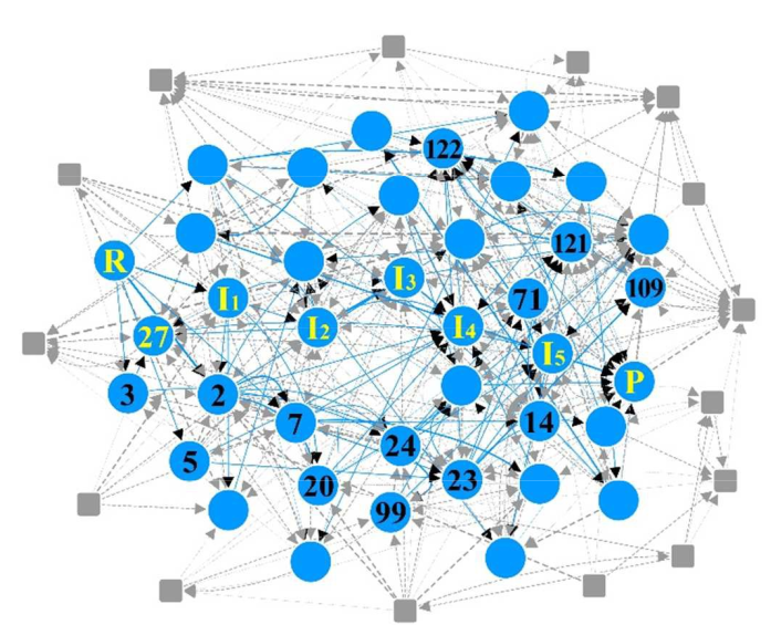
The ACErxn package holds a collection of tools for the generation of reaction networks from known reactant-product pairs [1]. A reaction network connects a reactant R and a product P via a large number of stable intermediate structures of the same stoichiometry.
ACErxn treats molecules as graphs, with the atoms as vertices and the bonds as edges. The 3D molecular geometries are only considered to determine the stability of generated intermediates. The AMS Python library PLAMS is used to optimize those geometries.
The minimal input requirements are:
Coordinates of all reactant and product molecules.
A set of atom indices for the active atoms in the reactants. The active atoms are the only atoms that can participate in bond breaking/forming.
Molecular charges of the reactants.
The ACErxn procedure consists of three steps, which by default are performed consecutively.
Intermediate generation: A set of intermediates is generated by enumeratively breaking and forming bonds in the reactant molecules.
Network creation: The intermediates are connected by elementary reactions, using filters based on the number of broken and formed bonds.
Network minimization: The most likely mechanisms from reactant to product are extracted, using shortest path algorithms [2] [3].
After running ACErxn, the reaction network information and the intermediates are stored as RKF files in a results folder. ACErxn is set up as a PLAMS-like library and uses PLAMS to generate a working folder with the default name plams_workdir. After running a single ACErxn job, the results folder is located inside this working folder, as plams_workdir/acerxn/acerxn.results.
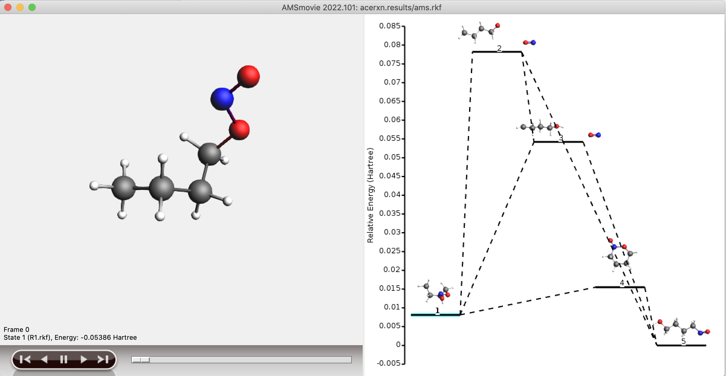
When the final step is completed (step 3), the shortest paths from reactant to product are stored as a separate network, in a separate folder containing RKF files. This folder is named plams_workdir/acerxn/shortest_paths. Both the full network and the shortest path network can be visualized using AMSMovie.
ACErxn can be used in two ways:
As a Python library.
As a command-line tool that reads a text input.
The command line tool is a wrapper around the Python library.
1.2. Simple example
In this example, a small reaction network is created for a simple unimolecular reaction.
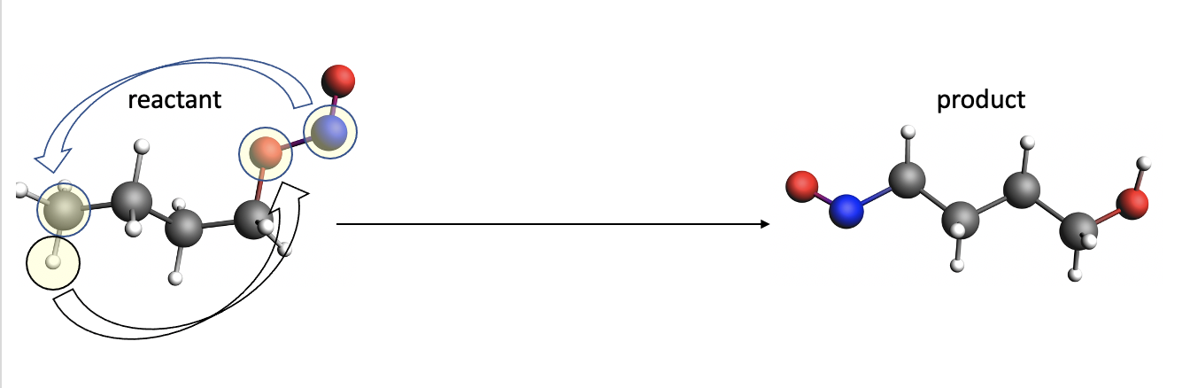
The set of active atoms needs to be selected as small as possible to keep the process of network generation efficient. In this case, we use chemical intuition to select only the atoms in transparent yellow circles as active atoms. In general, the number of selected active atoms should be no larger than 10.
The first example uses ACErxn as a Python library. It can be found in $AMSHOME/scripting/acerxn/examples/simple.
The reactant and product geometries need to be provided as separate files (e.g. as .xyz or .mol files). If no bonding information is provided in the files, then the bonds will be guessed (guess_bonds()).
import networkx as nx
import matplotlib.pyplot as plt
from scm.plams import Molecule, Settings
from scm.plams import init, finish
from scm.acerxn import Reactant, ACErxnNetwork


def main():
    """
    The main script
    """
    reactant_filenames = ["reactant.xyz"]
    product_filenames = ["product.xyz"]

    # Some user supplied info on the reactants
    molcharges = [0]
    active_atoms = [[0, 12, 13, 15]]

    # Create the reactant molecules
    reactants = [Molecule(fn) for fn in reactant_filenames]
    reactant = Reactant(reactants, active_atoms, molcharges)
    reactant.guess_fragments()

    # Create the product molecules
    products = [Molecule(fn) for fn in product_filenames]

    # Create the settings object
    settings = ACErxnNetwork.default_settings()

    # QM engine settings
    engine_settings = Settings()
    engine_settings.Mopac.Model = "PM6"
    settings.qmengine = engine_settings

    # Set up the ACE network
    network = ACErxnNetwork(reactant, products, settings=settings)

    # Now run the network, and create the reaction network
    init()
    network.generate()
    finish()

    # Optionally plot the resulting reaction network
    # nx.draw( network.graph, with_labels=True, node_color='white', edgecolors='blue', font_weight='bold', node_size=4000 )
    # plt.show()


if __name__ == "__main__":
    main()
The second example is a shell script that calls the ACErxn command line tool, and gives exactly the same result as the first example. In this case the reactant and product geometries are part of the input text.
#!/bin/sh

$AMSBIN/amspython $AMSHOME/scripting/scm/acerxn/run_acerxn.py << eor

system reactant0
  Atoms
              C       1.0700000000       2.4608000000       0.8738000000 active=True
              H       1.4267000000       2.9652000000       0.0001000000 active=False
              H       0.0000000000       2.4608000000       0.8738000000 active=False
              C       1.5833000000       1.0088000000       0.8738000000 active=False
              H       1.2266000000       0.5044000000       1.7474000000 active=False
              H       1.2266000000       0.5044000000       0.0001000000 active=False
              C       3.1233000000       1.0088000000       0.8738000000 active=False
              H       3.4800000000       0.0000000000       0.8739000000 active=False
              H       3.4800000000       1.5130000000       0.0000000000 active=False
              C       3.6367000000       1.7350000000       2.1310000000 active=False
              H       4.6201000000       1.3862000000       2.3678000000 active=False
              H       3.6666000000       2.7887000000       1.9471000000 active=False
              O       2.7590000000       1.4674000000       3.2278000000 active=True
              N       3.4288000000       1.6425000000       4.3984000000 active=True
              O       4.0183000000       1.7966000000       5.4285000000 active=False
              H       1.4267000000       2.9652000000       1.7474000000 active=True
  End
  BondOrders
     10 11 1
     1 16 1
     4 5 1
     7 10 1
     13 14 1
     1 3 1
     4 7 1
     7 8 1
     10 13 1
     7 9 1
     1 4 1
     10 12 1
     1 2 1
     4 6 1
     14 15 2.0
  End
  Charge 0
End

system product0_0
  Atoms
              C      -2.6271620000       2.3237140000       0.0648140000
              H      -2.2704890000       2.8281120000      -0.8088370000
              H      -3.6971620000       2.3237270000       0.0648140000
              C      -2.1138200000       3.0496700000       1.3222190000
              H      -2.4704580000       4.0584860000       1.3222100000
              H      -1.0438200000       3.0496400000       1.3222290000
              C      -2.6271850000       2.3237290000       2.5796230000
              H      -2.2705100000       2.8281250000       3.4532750000
              H      -3.6971850000       2.3237610000       2.5796150000
              C      -2.1138950000       0.8717870000       2.5796340000
              H      -2.0839500000       0.5040910000       3.5840260000
              H      -1.1304640000       0.8411400000       2.1591300000
              O      -3.0307730000       0.0154900000       1.8788390000
              N      -2.0980060000       0.9782090000      -0.0147070000
              O      -1.5860940000       0.5028570000      -1.0362940000
              H      -3.6277380000      -0.4600880000       2.4611260000
  End
  BondOrders
     1 2 1
     10 12 1
     4 7 1
     1 4 1
     13 16 1
     1 3 1
     4 6 1
     7 9 1
     7 8 1
     10 11 1
     4 5 1
     7 10 1
     10 13 1
     1 14 1
     14 15 2.0
  End
End

Engine Mopac
  Model PM6
EndEngine

eor
Both examples result in the same reaction network.
References