ZacrosResults
The ZacrosResults class was designed to take charge of the job folder after executing the ZacrosJob. It gathers the information from the output files and helps extract data of interest from them. Every ZacrosJob instance has an associated ZacrosResults instance created automatically on job creation and stored in its results attribute. This class extends the PLAMS Results class.
For our example (see use case system), the following lines of code show an example of how to use the ZacrosResults class:
1results = job.run()
2
3if( job.ok() ):
4 provided_quantities = results.provided_quantities()
5 print("nCO2 =", provided_quantities['CO2'])
6
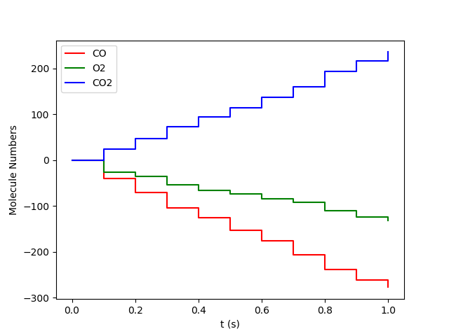
7 results.plot_molecule_numbers( results.gas_species_names() )
8 results.plot_lattice_states( results.lattice_states() )
9
10 pstat = results.get_process_statistics()
11 results.plot_process_statistics( pstat, key="number_of_events" )
Here, the ZacrosResults object results is created by calling the method run() of the corresponding ZacrosJob job (line 1).
Afterward, the method ok() is invoked to assure that the calculation finished appropriately (line 3), and only after that,
it is good to go to get information from the output files by using the ZacrosResults methods (lines 4-11).
As an example, the method provided quantities() returns the content of the zacros output file specnum_output.txt in the form of a dictionary. Thus, in line 5, we print out the number of CO2 molecules produced during the simulation. In addition to getting the information from the output files, the ZacrosResults class also offers some methods to plot the results directly, as shown in lines 7-11.
The execution of the block of code shown above produces the following information to the standard output:
[05.11|10:22:27] JOB plamsjob STARTED
[05.11|10:22:27] JOB plamsjob RUNNING
[05.11|10:22:27] JOB plamsjob FINISHED
[05.11|10:22:27] JOB plamsjob SUCCESSFUL
nCO2 = [0, 28, 57, 85, 118, 139, 161, 184, 212, 232, 264]
Notice the line corresponding to the number of CO2 molecules produced during the simulation. The rest of the functions generate the following figures:
results.plot_molecule_numbers( results.gas_species_names() )
results.plot_lattice_states( results.lattice_states() )
pstat = results.get_process_statistics()
results.plot_process_statistics( pstat, key="number_of_events" )
API
- class ZacrosResults(job: Job)
A Class for handling Zacros Results.
- get_zacros_version()
Returns the zacros’s version from the ‘general_output.txt’ file.
- get_reaction_network()
Returns the reactions from the ‘general_output.txt’ file.
- provided_quantities_names()
Returns the provided quantities headers from the
specnum_output.txtfile in a list. Below is shown an example of thespecnum_output.txtfor a zacros calculation.Entry Nevents Time Temperature Energy O* CO* O2 CO CO2 1 0 0.000E+00 5.00000E+02 -4.089E+01 11 12 0 0 0 2 88 1.000E-01 5.00000E+02 -7.269E+01 22 17 -21 -36 31 3 176 2.000E-01 5.00000E+02 -9.139E+01 29 19 -41 -71 64 4 247 3.000E-01 5.00000E+02 -1.041E+02 34 20 -57 -99 91
For this example, this function will return:
[ 'Entry', 'Nevents', 'Time', 'Temperature', 'Energy', 'O*', 'CO*', 'O2', 'CO', 'CO2' ]
- provided_quantities()
Returns the provided quantities from the
specnum_output.txtfile in a form of a dictionary. Below is shown an example of thespecnum_output.txtfor a zacros calculation.Entry Nevents Time Temperature Energy O* CO* O2 CO CO2 1 0 0.000E+00 5.00000E+02 -4.089E+01 11 12 0 0 0 2 88 1.000E-01 5.00000E+02 -7.269E+01 22 17 -21 -36 31 3 176 2.000E-01 5.00000E+02 -9.139E+01 29 19 -41 -71 64 4 247 3.000E-01 5.00000E+02 -1.041E+02 34 20 -57 -99 91
For this example, this function will return:
{
   "Entry":[1, 2, 3, 4],
   "Nevents":[0, 88, 176, 247],
   "Time":[0.000E+00, 1.000E-01, 2.000E-01, 3.000E-01],
   "Temperature":[5.00000E+02, 5.00000E+02, 5.00000E+02, 5.00000E+02],
   "Energy":[-4.089E+01, -7.269E+01, -9.139E+01, -1.041E+02],
   "O*":[11, 22, 29, 34],
   "CO*":[12, 17, 19, 20],
   "O2":[0, -21, -41, -57],
   "CO":[0, -36, -71, -99],
   "CO2":[0, 31, 64, 91]
}
- number_of_lattice_sites()
Returns the number of lattice sites from the ‘general_output.txt’ file.
- gas_species_names()
Returns the gas species names from the ‘general_output.txt’ file.
- surface_species_names()
Returns the surface species names from the ‘general_output.txt’ file.
- site_type_names()
Returns the site types from the ‘general_output.txt’ file.
- number_of_snapshots()
Returns the number of configurations from the ‘history_output.txt’ file.
- number_of_process_statistics()
Returns the number of process statistics from the ‘procstat_output.txt’ file.
- elementary_steps_names()
Returns the names of elementary steps from the ‘procstat_output.txt’ file.
- lattice_states(last=None)
Returns the configurations from the ‘history_output.txt’ file.
- last_lattice_state()
Returns the last configuration from the ‘history_output.txt’ file.
- average_coverage(last=5)
Returns a dictionary with the average coverage fractions using the last
lastlattice states, e.g.,{ "CO*":0.32, "O*":0.45 }.This function uses the information (provided quantities) from the
specnum_output.txtfile. So, it is quite fast. Below is shown an example of thespecnum_output.txtfor a zacros calculation.Entry Nevents Time Temperature Energy O* CO* O2 CO CO2 1 0 0.000E+00 5.00000E+02 -4.089E+01 11 12 0 0 0 2 88 1.000E-01 5.00000E+02 -7.269E+01 22 17 -21 -36 31 3 176 2.000E-01 5.00000E+02 -9.139E+01 29 19 -41 -71 64 4 247 3.000E-01 5.00000E+02 -1.041E+02 34 20 -57 -99 91
- average_coverage_fractions(last=5, site_names=None, species_symbols=None, normalize=False)
Returns a dictionary with the coverage fractions, e.g.,
{ "CO*":0.32, "O*":0.45 }.This function uses information from the “history_output.txt” file, which contains extensive details. While it may be a bit slow, it allows filtering by site names and species.
site_names– Name of the sites to be included, e.g.,["fcc","hcp"]species_symbols– Name of the species names to be included, e.g.,["H*","C*"]normalize– If set to False, the coverage fraction is normalized to the total number of sites. If True, only the total number of sites filtered by “site_names” are included.last– Number of lattice states to consider in the average, starting from the last one.
- average_site_coverage_fractions(last=5, site_names=None, species_symbols=None, normalize=False)
Returns a dictionary with the coverage fractions per site, e.g.,
{ "fcc":0.32, "hcp":0.45 }.This function uses information from the “history_output.txt” file, which contains extensive details. While it may be a bit slow, it allows filtering by site names and species.
site_names– Name of the sites to be included, e.g.,["fcc","hcp"]species_symbols– Name of the species names to be included, e.g.,["H*","C*"]normalize– If set to False, the coverage fraction is normalized to the total number of sites. If True, only the total number of sites filtered by “site_names” are included.last– Number of lattice states to consider in the average, starting from the last one.
- molecule_numbers(species_name, normalize_per_site=False)
The key ‘Time’ is included by default and includes the time in seconds. The other keys correspond to species selected by the parameter species_name and contain the number of molecules for the corresponding species. If normalize_per_site=True, these last values are divided by the number of sites on the surface. e.g.,
{ "Time":[0.0, 0.1, 0.2, ...], "O*":[5, 15, 20, ...], "CO2":[10, 25, 45, ...] }species_name– List of species names to show, e.g.,["CO*", "CO2"]normalize_per_site– Divides the molecule numbers by the total number of sites in the lattice.
- plot_lattice_states(data, pause=-1, show=True, ax=None, close=False, time_perframe=0.5, file_name=None, frames=None, markers=None, marker_size=1.0, colors=None, lattice_markers=None, lattice_color='0.8')
Uses Matplotlib to create an animation of the lattice states.
data– List of LatticeState objects to plotpause– After showing the figure, it will waitpause-seconds before refreshing.show– Enables showing the figure on the screen.ax– The axes of the plot. It contains most of the figure elements: Axis, Tick, Line2D, Text, Polygon, etc., and sets the coordinate system. See matplotlib.axes.close– Closes the figure window after pause time.time_perframe– Sets the time interval between frames in seconds.file_name– Saves the figures to the filefile_name-<id>(the corresponding id on the list replaces the<id>). The format is inferred from the extension, and by default,.pngis used.frames– Optional list where each frame artists list is appended. Useful formatplotlib.animation.ArtistAnimation.markers– List of marker styles used for site types.marker_size– Scale factor for marker area.colors– List of colors used for species.lattice_markers– List of marker styles used for lattice site types. IfNone,markersis used.lattice_color– Single color used to draw lattice sites, lattice unit-cell lines, and lattice connections.
- plot_molecule_numbers(species_name, pause=-1, show=True, ax=None, close=False, file_name=None, normalize_per_site=False, derivative=False)
uses Matplotlib to create an animation of the Molecule Numbers.
species_name– List of species names to show, e.g.,["CO*", "CO2"]pause– After showing the figure, it will waitpause-seconds before refreshing. This can be used for crude animation.show– Enables showing the figure on the screen.ax– The axes of the plot. It contains most of the figure elements: Axis, Tick, Line2D, Text, Polygon, etc., and sets the coordinate system. See matplotlib.axes.close– Closes the figure window after pause time.file_name– Saves the figure to the filefile_name. The format is inferred from the extension, and by default,.pngis used.normalize_per_site– Divides the molecule numbers by the total number of sites in the lattice.derivative– Plots the first derivative.
- get_process_statistics()
Returns the statistics from the ‘procstat_output.txt’ file in a form of a list of dictionaries. Below is shown an example of the
procstat_output.txtfor a zacros calculation.Overall CO_ads O2_react_ads CO_oxi configuration 1 0 0.00 0.000 0.000 0.000 0.000 0 0 0 0 configuration 2 250 0.01 0.039 0.043 0.044 0.000 250 108 118 24
For this example, this function will return:
[
  {
    'configuration_number': 1,
    'total_number_of_events': 0,
    'time': 0.0,
    'average_waiting_time': {
                              'CO_ads': 0.0,
                              'O2_react_ads': 0.0,
                              'CO_oxi': 0.0
                            },
    'number_of_events': {
                          'CO_ads': 0,
                          'O2_react_ads': 0,
                          'CO_oxi': 0
                        },
    'occurence_frequency': {
                             'CO_ads': 0.0,
                             'O2_react_ads': 0.0,
                             'CO_oxi': 0.0
                           }
  },
  {
    'configuration_number': 2,
    'total_number_of_events': 250,
    'time': 0.01,
    'average_waiting_time': {
                              'CO_ads': 0.043
                              'O2_react_ads': 0.044
                              'CO_oxi': 0.0
                            },
    'number_of_events': {
                          'CO_ads': 108,
                          'O2_react_ads': 118,
                          'CO_oxi': 24
                        },
    'occurence_frequency': {
                             'CO_ads': 10800.0,
                             'O2_react_ads': 11800.0,
                             'CO_oxi': 2400.0
                           }
  }
]
The
occurence_frequencyis calculated asnumber_of_events/time.
- plot_process_statistics(data, key, log_scale=False, pause=-1, show=True, ax=None, close=False, file_name=None)
Uses Matplotlib to create an animation of the process statistics.
data– List of process statistics to plot. See functionget_process_statistics().key– Key to plot, e.g.,'average_waiting_time','average_waiting_time'. See functionget_process_statistics().log_scale– Use log scale for the x axis.pause– After showing the figure, it will waitpause-seconds before refreshing.show– Enables showing the figure on the screen.ax– The axes of the plot. It contains most of the figure elements: Axis, Tick, Line2D, Text, Polygon, etc., and sets the coordinate system. See matplotlib.axes.close– Closes the figure window after pause time.file_name– Saves the figures to the filefile_name-<id>(the corresponding id on the list replaces the<id>). The format is inferred from the extension, and by default,.pngis used.
- turnover_frequency(nbatch=20, confidence=0.99, ignore_nbatch=1, species_name=None, provided_quantities=None)
Returns the TOF (mol/sec/site) calculated by the batch-means stopping method. See Hashemi et al., J.Chem. Phys. 144, 074104 (2016)
nbatch– Number of batches to use.confidence– Confidence level to use in the criterion to determine if the steady-state was reached.ignore_nbatch– Number of batches to ignore during the averaging in the calculation of the TOF.
The simulation output is divided into an ensemble of contiguous batches where the TOF is computed. The average value and the standard deviation of the TOF ensemble are evaluated as follows:
\[<TOF> = \frac{1}{n}\sum_{i=1}^n TOF_i \qquad \sigma_{TOF}\sqrt{\frac{1}{n-1}\sum_{i=1}^n\left(TOF_i-<TOF>\right)}\]where \(n = \text{nbatch}\). Confidence intervals are estimated to assess the steady-state behavior of the simulation:
\[<TOF>\pm t_{n-1,1-\frac{\delta}{2}}\frac{\sigma_{TOF}}{\sqrt{n}}\]The function returns True when the steady-state is reached. This happens if the following equation is satisfied:
\[t_{n-1,1-\frac{\delta}{2}}\frac{\sigma_{TOF}}{\sqrt{n}} \lt \epsilon\]Here the convergence criteria is \(\epsilon=1-\text{confidence}\)