LatticeState
A significant result from a KMC simulation is how the different sites in the lattice are populated as a function of time.
During a Zacros simulation, Zacros takes snapshots of the lattice state and writes them in the file history_output.txt.
Parallelly pyZacros stores each snapshot as a LatticeState object (see ZacrosResults) for further analysis and/or use
on the python side. Another important application of LatticeState objects is that they can be used as initial states, either
as objects from a previous simulation or built from scratch.
For our example (see use case system), we will use the LatticeState class to build a
lattice state from scratch, and use it as the initial state.
Note
pyZacros (and Zacros) will start with an empty lattice if not stated otherwise.
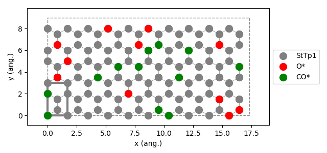
We are going to make the initial state as a randomly populated lattice by CO* and O* with a given coverage:
1# LatticeState setup (initial state)
2ist = pz.LatticeState(lat, surface_species=spl.surface_species())
3ist.fill_sites_random(site_name='StTp1', species='CO*', coverage=0.1)
4ist.fill_sites_random(site_name='StTp1', species='O*', coverage=0.1)
5
6print(ist)
7
8ist.plot()
Similarly to the other classes, the function print() (see line 6) allows taking a look at the Zacros code that
will be internally generated, which for this example is the following:
initial_state
  # species * CO* O*
  # species_numbers
  #   - CO*  12
  #   - O*  11
  seed_on_sites CO* 1
  seed_on_sites CO* 4
  seed_on_sites O* 6
  seed_on_sites O* 10
  seed_on_sites O* 20
  seed_on_sites CO* 30
  seed_on_sites CO* 43
  seed_on_sites O* 48
  seed_on_sites O* 52
  seed_on_sites CO* 55
  seed_on_sites O* 58
  seed_on_sites CO* 62
  seed_on_sites CO* 69
  seed_on_sites CO* 70
  seed_on_sites O* 72
  seed_on_sites CO* 73
  seed_on_sites CO* 78
  seed_on_sites CO* 93
  seed_on_sites O* 99
  seed_on_sites O* 106
  seed_on_sites O* 109
  seed_on_sites O* 110
  seed_on_sites CO* 115
end_initial_state
Please consult Zacros’ user guide ($AMSHOME/scripting/scm/pyzacros/doc/ZacrosManual.pdf) for more details about the specific meaning of the keywords used in the previous lines.
Finally, to visualize the lattice you can make use of the function plot() (see line 8). The result is as follows:
Note
To visualize the previous figure, be sure you have matplotlib installed.
API
- class LatticeState(lattice, surface_species, initial=True, add_info=None)
LatticeState class represents the lattice state at a specific time during a Zacros simulation. Fundamentally contains information about which species populate the particular sites in the lattice. LatticeStates objects can be used for visualization/analysis purposes or as initial states for a new ZacrosJob.
lattice– Reference latticesurface_species– List of allowed surface species, e.g.,[ Species("H*"), Species("O*") ]initial– If True, it indicates that the state represents an initial state. This is used to create the Zacros input files. If the state is an initial state the corresponding block in the Zacros input files isinitial_state ... end_initial_state, otherwisestate ... end_stateis used.add_info– A dictionary containing additional information. For example,self.add_info['time']will be used as part of the title in the figure generated by the functionplot().
- empty()
Returns True if the state is empty
- number_of_filled_sites()
Returns the number of filled sites on the lattice
- fill_site(site_number, species, update_species_numbers=True)
Fills the
site_numbersite with the speciesspeciessite_number– Integer number indicating the site id to be filled.species– Species to be used to fill the site, e.g.,Species("O2*"), or"O2*".update_species_numbers– Forces to update the statistics about the number of species adsorbed in the lattice. For better performance, it would be wise to set it to False if a massive number of species are going to be added (one by one) using this function.
- fill_sites_random(site_name, species, coverage, neighboring=None)
Fills the named sites
site_namerandomly with the speciesspeciesby keeping a coverage given bycoverage. Coverage is defined relative to the available empty sites. Neighboring can be specified if the sites are not neighboring linearly, but are branched or cyclical.site_name– Name of the sites to be filled, e.g.,["fcc","hcp"]species– Species to be used to fill the site, e.g.,Species("O2*"), or"O2*".coverage– A number between 0.0 and 1.0 represents the expected coverage. The function will try to generate coverage as close as possible to this number.neighboring– Neighboring relations associated to the sitessite_name, e.g.,[[0,2],[1,2]].
- fill_all_sites(site_name, species)
Fills all available named sites
site_namewith the speciesspecies.site_name– Name of the sites to be filled, e.g.,["fcc","hcp"]species– Species to be used to fill the site, e.g.,Species("O2*"), or"O2*".
- coverage_fractions(site_names=None, species_symbols=None, normalize=False)
Returns a dictionary with the coverage fractions, e.g.,
{ "CO*":0.32, "O*":0.45 }.This function uses information from the “history_output.txt” file, which contains extensive details. While it may be a bit slow, it allows filtering by site names and species.
site_names– Name of the sites to be included, e.g.,["fcc","hcp"]species_symbols– Name of the species names to be included, e.g.,["H*","C*"]normalize– If set to False, the coverage fraction is normalized to the total number of sites. If True, only the total number of sites filtered by “site_names” are included.
- site_coverage_fractions(site_names=None, species_symbols=None, normalize=False)
Returns a dictionary with the coverage fractions per site, e.g.,
{ "fcc":0.32, "hcp":0.45 }.This function uses information from the “history_output.txt” file, which contains extensive details. While it may be a bit slow, it allows filtering by site names and species.
site_names– Name of the sites to be included, e.g.,["fcc","hcp"]species_symbols– Name of the species names to be included, e.g.,["H*","C*"]normalize– If set to False, the coverage fraction is normalized to the total number of sites. If True, only the total number of sites filtered by “site_names” are included.
- plot(pause=-1, show=True, ax=None, close=False, show_sites_ids=False, file_name=None, markers=None, marker_size=1.0, colors=None, lattice_markers=None, lattice_color='0.8')
Uses matplotlib to visualize the lattice state
pause– After showing the figure, it will waitpause-seconds before refreshing. This can be used for crude animation.show– Enables showing the figure on the screen.ax– The axes of the plot. It contains most of the figure elements: Axis, Tick, Line2D, Text, Polygon, etc., and sets the coordinate system. See matplotlib.axes.close– Closes the figure window after pause time.show_sites_ids– Shows the binding sites id on the figure.file_name– Saves the figure to the filefile_name. The format is inferred from the extension, and by default,.pngis used.markers– List of marker styles used for site types.marker_size– Scale factor for marker area.colors– List of colors used for species.lattice_markers– List of marker styles used for lattice site types. IfNone,markersis used.lattice_color– Single color used to draw lattice sites, lattice unit-cell lines, and lattice connections.