Active Learning: Committee Uncertainties and ReactionBoost for a Gasphase Reaction

MLPotential Active Learning ParAMS M3GNet ReactionBoost Committee Models

Use committee-model uncertainties and ReactionBoost molecular dynamics to sample a reactive pathway, retrain custom M3GNet models, and improve the reaction barrier for propene hydration.

Downloads: Notebook | Script ?

Requires: AMS2026 or later

Required AMS Packages: m3gnet

Related examples

• Active Learning: Li-Vacancy Diffusion NEB in LiTiS2

• Active Learning: Single-Molecule Setup and Run

• M3GNet Custom Model

Related tutorials

• Simple Active Learning tutorial

• Targeted MD tutorial

Related documentation

• Simple Active Learning Python API

• Molecular Dynamics task

• MLPotential engine

Initial imports

import scm.plams as plams
from scm.simple_active_learning import SimpleActiveLearningJob
from scm.reactmap.tools import reorder_plams_mol
import matplotlib.pyplot as plt
from scm.input_classes import drivers, engines
from scm.base import Units
import scm.params as params
import os
import numpy as np

plams.init()

PLAMS working folder: /path/to/plams_workdir.002

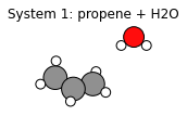
system1 = plams.from_smiles("CC=C", forcefield="uff")  # propene

# add a water molecule *at least* 1 angstrom away from all propene atoms
system1.add_molecule(plams.from_smiles("O"), margin=1)

for at in system1:
    at.properties = plams.Settings()
system1.delete_all_bonds()

plams.plot_molecule(system1)
plt.title("System 1: propene + H2O");

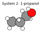
system2 = plams.from_smiles("CCCO")  # 1-propanol
for at in system2:
    at.properties = plams.Settings()
system2.delete_all_bonds()

# reorder atoms in system2 to match the order in system1
# this only takes bond breaking and forming into account, the order is not guaranteed to match exactly for all atoms
system2 = reorder_plams_mol(system1, system2)

# Rotate system2 so that the RMSD with respect to system1 is minimized
system2.align2mol(system1)

plams.plot_molecule(system2)
plt.title("System 2: 1-propanol");

# sanity-check that at least the order of elements is identical
assert list(system1.symbols) == list(system2.symbols), f"Something went wrong!"

Note that this does not guarantee that the atom order is completely the same. For example the order of the hydrogen atoms in the CH3 group might be different. This means that we cannot just run NEB directly. So let’s first run MD ReactionBoost.

Initial Reaction Boost to get reactant and product

Engine settings

Here we use e_up to refer to the M3GNet Universal Potential.

For the ADF DFT engine we set an electronic temperature and the OptimizeSpinRound option. This helps with SCF convergence, and can converge the SCF to a different spin state when applicable.

e_up = engines.MLPotential()
e_up.Model = "M3GNet-UP-2022"

e_dft = engines.ADF()
e_dft.XC.GGA = "PBE"
e_dft.XC.Dispersion = "GRIMME3 BJDAMP"
e_dft.Basis.Type = "TZP"
e_dft.Unrestricted = True
e_dft.Occupations = "ElectronicTemperature=300 OptimizeSpinRound=0.05"

def set_reaction_boost(driver, nsteps=3000):
    driver.Task = "MolecularDynamics"
    md = driver.MolecularDynamics
    md.InitialVelocities.Temperature = 100
    md.NSteps = nsteps
    md.ReactionBoost.Type = "Pair"
    md.ReactionBoost.BondBreakingRestraints.Type = "Erf"
    md.ReactionBoost.BondBreakingRestraints.Erf.MaxForce = 0.05
    md.ReactionBoost.BondMakingRestraints.Type = "Erf"
    md.ReactionBoost.BondMakingRestraints.Erf.MaxForce = 0.12
    md.ReactionBoost.InitialFraction = 0.05
    md.ReactionBoost.Change = "LogForce"
    md.ReactionBoost.NSteps = nsteps
    md.ReactionBoost.TargetSystem[0] = "final"
    md.Trajectory.SamplingFreq = 10
    md.Trajectory.WriteBonds = False
    md.Trajectory.WriteMolecules = False
    md.TimeStep = 0.25
    md.Thermostat[0].Tau = 5
    md.Thermostat[0].Temperature = [100.0]
    md.Thermostat[0].Type = "Berendsen"

def get_reaction_boost_job(
    engine, molecule, name: str = "reaction_boost"
) -> plams.AMSJob:
    d = drivers.AMS()
    set_reaction_boost(d)
    d.Engine = engine
    job = plams.AMSJob(settings=d, name=name, molecule=molecule)
    job.settings.runscript.nproc = 1
    return job

molecule_dict = {"": system1, "final": system2}
prelim_job = get_reaction_boost_job(e_up, molecule_dict, "prelim_md")

prelim_job.run();

[03.04|14:11:30] JOB prelim_md STARTED
[03.04|14:11:30] JOB prelim_md RUNNING
[03.04|14:12:19] JOB prelim_md FINISHED
[03.04|14:12:19] JOB prelim_md SUCCESSFUL

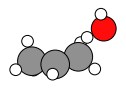
Let’s check that the final molecule corresponds to the target system (1-propanol):

engine_energies = prelim_job.results.get_history_property("EngineEnergy")
N_frames = len(engine_energies)
max_index = np.argmax(engine_energies)
reactant_index = max(0, max_index - 50)  # zero-based
system1_correct_order = prelim_job.results.get_history_molecule(reactant_index + 1)
system1_correct_order.delete_all_bonds()
plams.plot_molecule(system1_correct_order)

product_index = min(max_index + 50, N_frames - 1)  # zero-based
system2_correct_order = prelim_job.results.get_history_molecule(product_index + 1)
system1_correct_order.delete_all_bonds()
plams.plot_molecule(system2_correct_order)

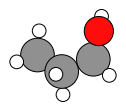
We now have the product molecule with the correct atom order, which means we can run an initial NEB with M3GNet and compare to the DFT reference:

Initial NEB calculation

molecule_dict = {"": system1_correct_order, "final": system2_correct_order}

def get_neb_job(engine, name: str = "neb") -> plams.AMSJob:
    d = drivers.AMS()
    d.Task = "NEB"
    d.GeometryOptimization.Convergence.Quality = "Basic"
    d.NEB.Images = 12
    d.Engine = engine

    neb_job = plams.AMSJob(name=name, settings=d, molecule=molecule_dict)
    return neb_job

neb_job = get_neb_job(e_up, name="neb_up")
neb_job.run();

[03.04|14:14:19] JOB neb_up STARTED
[03.04|14:14:19] JOB neb_up RUNNING
[03.04|14:14:45] JOB neb_up FINISHED
[03.04|14:14:46] JOB neb_up SUCCESSFUL

Let’s then replay with the ADF DFT engine.

def get_replay_job(rkf, name="replay"):
    d_replay = drivers.AMS()
    d_replay.Task = "Replay"
    d_replay.Replay.File = os.path.abspath(rkf)
    d_replay.Properties.Gradients = True
    d_replay.Engine = e_dft

    replay_job = plams.AMSJob(name=name, settings=d_replay)
    return replay_job

replay_job = get_replay_job(neb_job.results.rkfpath(), "replay_neb")
replay_job.run();

[03.04|14:14:51] JOB replay_neb STARTED
[03.04|14:14:51] JOB replay_neb RUNNING
[03.04|14:15:57] JOB replay_neb FINISHED
[03.04|14:15:58] JOB replay_neb SUCCESSFUL

def get_relative_energies(neb_job):
    e = neb_job.results.get_neb_results()["Energies"]
    e = np.array(e) - np.min(e)
    e *= Units.conversion_factor("hartree", "eV")
    return e


def plot_neb_comparison(neb_job, replay_job, legend=None, title=None):
    energies_up = get_relative_energies(neb_job)
    energies_dft = get_relative_energies(replay_job)
    fig, ax = plt.subplots()
    ax.plot(energies_up)
    ax.plot(energies_dft)
    ax.legend(legend or ["M3GNet-UP-2022", "DFT singlepoints"])
    ax.set_ylabel("Relative energy (eV)")
    ax.set_title(title or "Reaction path water+propene -> 1-propanol")
    return ax

plot_neb_comparison(neb_job, replay_job);

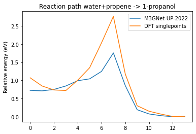
So we can see that either M3GNet-UP-2022 underestimates the barrier or it NEB path is different from the DFT one. Let’s use these datapoints as a starting point for the active learning.

Simple Active Learning using Uncertainties

Create the initial reference data

Let’s run replay on some of the frames from the prelim_md reaction boost job:

replay_md = get_replay_job(prelim_job.results.rkfpath(), "replay_md")
N_frames_to_replay = 10
replay_md.settings.input.Replay.Frames = list(
    np.linspace(reactant_index, product_index, N_frames_to_replay, dtype=np.int64)
)
replay_md.run();

[03.04|14:16:22] JOB replay_md STARTED
[03.04|14:16:22] JOB replay_md RUNNING
[03.04|14:17:11] JOB replay_md FINISHED
[03.04|14:17:12] JOB replay_md SUCCESSFUL

To construct our reference data, we will include both the NEB and MD frames from our replay calculations.

yaml_dir = "my_neb_data"
ri = params.ResultsImporter.from_ase()  # use ASE units
ri.add_trajectory_singlepoints(
    replay_job.results.rkfpath(),
    properties=["energy", "forces"],
    data_set="training_set",
)
ri.add_trajectory_singlepoints(
    replay_md.results.rkfpath(),
    properties=["energy", "forces"],
    data_set="training_set",
    indices=list(range(1, N_frames_to_replay - 1)),
)
ri.add_trajectory_singlepoints(
    replay_md.results.rkfpath(),
    properties=["energy", "forces"],
    indices=[0, N_frames_to_replay - 1],
    data_set="validation_set",
)
ri.store(yaml_dir, backup=False)

['my_neb_data/job_collection.yaml',
 'my_neb_data/results_importer_settings.yaml',
 'my_neb_data/training_set.yaml',
 'my_neb_data/validation_set.yaml']

When we have initial reference data like this, it’s often most convenient to run a separate ParAMS training before starting the active learning.

This lets us sanity-check the training parameters, and more easily try different Active Learning settings without having to retrain the initial model every time.

def get_params_job(yaml_dir, load_model=None, name="paramsjob"):
    committee_size = 2
    paramsjob = params.ParAMSJob.from_yaml(yaml_dir, use_relative_paths=True, name=name)
    paramsjob.settings.input.Task = "MachineLearning"
    ml = paramsjob.settings.input.MachineLearning
    ml.Backend = "M3GNet"
    if load_model:
        ml.LoadModel = load_model
        ml.MaxEpochs = 200
        ml.M3GNet.LearningRate = 5e-4
    else:
        ml.M3GNet.Model = "Custom"
        ml.M3GNet.Custom.NumNeurons = 32
        ml.MaxEpochs = 300
        ml.M3GNet.LearningRate = 1e-3

    ml.CommitteeSize = committee_size
    paramsjob.settings.input.ParallelLevels.CommitteeMembers = committee_size

    return paramsjob

paramsjob = get_params_job(yaml_dir, name="custom_initial_training")
paramsjob.run();

[03.04|14:17:48] JOB custom_initial_training STARTED
[03.04|14:17:48] JOB custom_initial_training RUNNING
[03.04|14:20:57] JOB custom_initial_training FINISHED
[03.04|14:20:57] JOB custom_initial_training SUCCESSFUL





<scm.params.plams.paramsjob.ParAMSResults at 0x7fae1d5130a0>

Set up the active learning job

Here the key new setting is the ReasonableSimulationCriteria.GradientsUncertainty. This setting will cause the MD simulation to instantly stop if the uncertainty is greater than 1.0 eV/angstrom.

This is useful since the ML model is unlikely to give good predictions for the new types of structures encountered during the reactive MD.

In the summary log, such an event will be marked as “FAILED” with the reason “GRADIENTS_UNCERTAINTY”.

In order to use ML uncertainties, you need to train a committee model with at least 2 members. Here we set the committee size to 2. We also choose to train the 2 committee members in parallel. By default, they would be trained in sequence.

It is a good idea to train them in parallel if you have the computational resources to do so (for example, enough GPU memory).

When using uncertainty-based criteria, you may consider increasing the MaxAttemptsPerStep. Here, we stick with the default value of 15.

d_al = drivers.SimpleActiveLearning()
d_al.ActiveLearning.InitialReferenceData.Load.FromPreviousModel = True
d_al.ActiveLearning.Steps.Type = "Geometric"
d_al.ActiveLearning.Steps.Geometric.NumSteps = 5
d_al.ActiveLearning.Steps.Geometric.Start = 10
d_al.ActiveLearning.ReasonableSimulationCriteria.GradientsUncertainty.Enabled = True
d_al.ActiveLearning.ReasonableSimulationCriteria.GradientsUncertainty.MaxValue = (
    1.0  # eV/ang
)
d_al.ActiveLearning.SuccessCriteria.Forces.MinR2 = 0.4
d_al.ActiveLearning.MaxReferenceCalculationsPerAttempt = 3
d_al.ActiveLearning.MaxAttemptsPerStep = 15
d_al.MachineLearning.Backend = "M3GNet"
d_al.MachineLearning.LoadModel = os.path.abspath(paramsjob.results.path)
d_al.MachineLearning.CommitteeSize = 2
d_al.MachineLearning.MaxEpochs = 120
d_al.MachineLearning.M3GNet.LearningRate = 5e-4
d_al.MachineLearning.RunAMSAtEnd = False
d_al.ParallelLevels.CommitteeMembers = 2
set_reaction_boost(d_al)
d_al.Engine = e_dft

sal_job = SimpleActiveLearningJob(name="sal", driver=d_al, molecule=molecule_dict)
print(sal_job.get_input())

ActiveLearning
  InitialReferenceData
    Load
      FromPreviousModel True
    End
... output trimmed ....
              H       2.5409431029       2.4889805122       0.3092516933
              H       0.4762175222      -0.1339653764       1.8246483976
  End
End

sal_job.run(watch=True)

[03.04|14:22:56] JOB sal STARTED
[03.04|14:22:56] JOB sal RUNNING
[03.04|14:22:58] Simple Active Learning 2024.101,  Nodes: 1, Procs: 8
[03.04|14:23:01] Composition of main system: C3H8O
[03.04|14:23:01] All REFERENCE calculations will be performed with the following ADF engine:
... output trimmed ....
[03.04|16:50:10] Rerunning the simulation with the final parameters...
[03.04|16:51:52] Copying final_production_simulation/ams.rkf to ams.rkf
[03.04|16:51:52] Goodbye!
[03.04|16:51:53] JOB sal FINISHED
[03.04|16:51:53] JOB sal SUCCESSFUL





<scm.simple_active_learning.plams.simple_active_learning_job.SimpleActiveLearningResults at 0x7fae1d9a56d0>

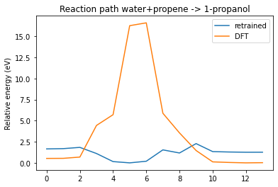
Above we see that during step 5, several attempts failed with the message GRADIENTS_UNCERTAINTY. This is the step during which the actual reaction happens. We do not know the exact time at which the reaction occurs (since the ReactionBoost gradually increases the applied force).

In such a case it is useful to have the GradientsUncertainty criterion enabled. This will immediately stop the simulation when the uncertainty is too high and follow it with a retraining of the model.

New NEB validation

Let’s now evaluate with a second-round NEB and replay. sal_job.results.get_production_engine_settings() returns the engine settings in the PLAMS Settings format. Let’s first convert it to a PISA Engine:

def settings2engine(settings):
    temporary_d = drivers.AMS.from_settings(settings)
    return temporary_d.Engine

e_new = settings2engine(sal_job.results.get_production_engine_settings())

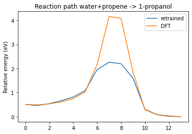
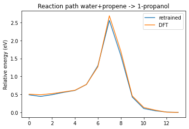
Let’s now create our own active learning loop for NEB where we run the NEB calculation with our trained potential, replay, add points to training set, retrain, rerun NEB etc.

We need to do this since MD SAL may not exactly sample the minimum energy path.

n_loop = 3
ri = params.ResultsImporter.from_yaml(sal_job.results.get_reference_data_directory())
params_results_dir = sal_job.results.get_params_results_directory()
for i in range(n_loop):
    neb = get_neb_job(e_new, f"new_neb{i}")
    neb.run()
    replay = get_replay_job(neb.results.rkfpath(), name=f"new_replay{i}")
    replay.run()
    plot_neb_comparison(neb, replay, legend=["retrained", "DFT"])
    yaml_dir = f"new_yaml_dir{i}"
    ri.add_trajectory_singlepoints(
        replay.results.rkfpath(), properties=["energy", "forces"]
    )
    ri.store(yaml_dir, backup=False)
    paramsjob = get_params_job(
        yaml_dir, load_model=params_results_dir, name=f"new_params{i}"
    )
    paramsjob.run()
    e_new = settings2engine(paramsjob.results.get_production_engine_settings())
    params_results_dir = os.path.abspath(paramsjob.results.path)

[03.04|16:53:38] JOB new_neb0 STARTED
[03.04|16:53:38] JOB new_neb0 RUNNING
[03.04|16:55:00] JOB new_neb0 FINISHED
[03.04|16:55:01] JOB new_neb0 SUCCESSFUL
[03.04|16:55:01] JOB new_replay0 STARTED
... output trimmed ....
[03.04|17:21:25] JOB new_replay2 SUCCESSFUL
[03.04|17:21:26] JOB new_params2 STARTED
[03.04|17:21:26] JOB new_params2 RUNNING
[03.04|17:29:30] JOB new_params2 FINISHED
[03.04|17:29:30] JOB new_params2 SUCCESSFUL

See also

Related examples

• Active Learning: Li-Vacancy Diffusion NEB in LiTiS2

• Active Learning: Single-Molecule Setup and Run

• M3GNet Custom Model

Related tutorials

• Simple Active Learning tutorial

• Targeted MD tutorial

Related documentation

• Simple Active Learning Python API

• Molecular Dynamics task

• MLPotential engine

Python Script

#!/usr/bin/env python
# coding: utf-8

# ## Initial imports

import scm.plams as plams
from scm.simple_active_learning import SimpleActiveLearningJob
from scm.reactmap.tools import reorder_plams_mol
import matplotlib.pyplot as plt
from scm.input_classes import drivers, engines
from scm.base import Units
import scm.params as params
import os
import numpy as np


plams.init()


system1 = plams.from_smiles("CC=C", forcefield="uff")  # propene

# add a water molecule *at least* 1 angstrom away from all propene atoms
system1.add_molecule(plams.from_smiles("O"), margin=1)

for at in system1:
    at.properties = plams.Settings()
system1.delete_all_bonds()

plams.plot_molecule(system1)
plt.title("System 1: propene + H2O")
plt.gcf().savefig("picture1.png")
plt.clf()


system2 = plams.from_smiles("CCCO")  # 1-propanol
for at in system2:
    at.properties = plams.Settings()
system2.delete_all_bonds()

# reorder atoms in system2 to match the order in system1
# this only takes bond breaking and forming into account, the order is not guaranteed to match exactly for all atoms
system2 = reorder_plams_mol(system1, system2)

# Rotate system2 so that the RMSD with respect to system1 is minimized
system2.align2mol(system1)

plams.plot_molecule(system2)
plt.title("System 2: 1-propanol")
plt.gcf().savefig("picture2.png")
plt.clf()


# sanity-check that at least the order of elements is identical
assert list(system1.symbols) == list(system2.symbols), f"Something went wrong!"


# Note that this does not guarantee that the atom order is completely the same.
# For example the order of the hydrogen atoms in the CH3 group might be different.
# This means that we cannot just run NEB directly. So let's first run MD ReactionBoost.

# ## Initial Reaction Boost to get reactant and product

# ### Engine settings
#
# Here we use ``e_up`` to refer to the M3GNet Universal Potential.
#
# For the ADF DFT engine we set an electronic temperature and the OptimizeSpinRound option. This helps with SCF convergence, and can converge the SCF to a different spin state when applicable.

e_up = engines.MLPotential()
e_up.Model = "M3GNet-UP-2022"

e_dft = engines.ADF()
e_dft.XC.GGA = "PBE"
e_dft.XC.Dispersion = "GRIMME3 BJDAMP"
e_dft.Basis.Type = "TZP"
e_dft.Unrestricted = True
e_dft.Occupations = "ElectronicTemperature=300 OptimizeSpinRound=0.05"


def set_reaction_boost(driver, nsteps=3000):
    driver.Task = "MolecularDynamics"
    md = driver.MolecularDynamics
    md.InitialVelocities.Temperature = 100
    md.NSteps = nsteps
    md.ReactionBoost.Type = "Pair"
    md.ReactionBoost.BondBreakingRestraints.Type = "Erf"
    md.ReactionBoost.BondBreakingRestraints.Erf.MaxForce = 0.05
    md.ReactionBoost.BondMakingRestraints.Type = "Erf"
    md.ReactionBoost.BondMakingRestraints.Erf.MaxForce = 0.12
    md.ReactionBoost.InitialFraction = 0.05
    md.ReactionBoost.Change = "LogForce"
    md.ReactionBoost.NSteps = nsteps
    md.ReactionBoost.TargetSystem[0] = "final"
    md.Trajectory.SamplingFreq = 10
    md.Trajectory.WriteBonds = False
    md.Trajectory.WriteMolecules = False
    md.TimeStep = 0.25
    md.Thermostat[0].Tau = 5
    md.Thermostat[0].Temperature = [100.0]
    md.Thermostat[0].Type = "Berendsen"


def get_reaction_boost_job(engine, molecule, name: str = "reaction_boost") -> plams.AMSJob:
    d = drivers.AMS()
    set_reaction_boost(d)
    d.Engine = engine
    job = plams.AMSJob(settings=d, name=name, molecule=molecule)
    job.settings.runscript.nproc = 1
    return job


molecule_dict = {"": system1, "final": system2}
prelim_job = get_reaction_boost_job(e_up, molecule_dict, "prelim_md")


prelim_job.run()
# Let's check that the final molecule corresponds to the target system (1-propanol):

#

engine_energies = prelim_job.results.get_history_property("EngineEnergy")
N_frames = len(engine_energies)
max_index = np.argmax(engine_energies)
reactant_index = max(0, max_index - 50)  # zero-based
system1_correct_order = prelim_job.results.get_history_molecule(reactant_index + 1)
system1_correct_order.delete_all_bonds()
plams.plot_molecule(system1_correct_order)


product_index = min(max_index + 50, N_frames - 1)  # zero-based
system2_correct_order = prelim_job.results.get_history_molecule(product_index + 1)
system1_correct_order.delete_all_bonds()
plams.plot_molecule(system2_correct_order)


# We now have the product molecule with the correct atom order, which means we can run an initial NEB with M3GNet and compare to the DFT reference:

# ## Initial NEB calculation

molecule_dict = {"": system1_correct_order, "final": system2_correct_order}


def get_neb_job(engine, name: str = "neb") -> plams.AMSJob:
    d = drivers.AMS()
    d.Task = "NEB"
    d.GeometryOptimization.Convergence.Quality = "Basic"
    d.NEB.Images = 12
    d.Engine = engine

    neb_job = plams.AMSJob(name=name, settings=d, molecule=molecule_dict)
    return neb_job


neb_job = get_neb_job(e_up, name="neb_up")
neb_job.run()


# Let's then replay with the ADF DFT engine.


def get_replay_job(rkf, name="replay"):
    d_replay = drivers.AMS()
    d_replay.Task = "Replay"
    d_replay.Replay.File = os.path.abspath(rkf)
    d_replay.Properties.Gradients = True
    d_replay.Engine = e_dft

    replay_job = plams.AMSJob(name=name, settings=d_replay)
    return replay_job


replay_job = get_replay_job(neb_job.results.rkfpath(), "replay_neb")
replay_job.run()


def get_relative_energies(neb_job):
    e = neb_job.results.get_neb_results()["Energies"]
    e = np.array(e) - np.min(e)
    e *= Units.conversion_factor("hartree", "eV")
    return e


def plot_neb_comparison(neb_job, replay_job, legend=None, title=None):
    energies_up = get_relative_energies(neb_job)
    energies_dft = get_relative_energies(replay_job)
    fig, ax = plt.subplots()
    ax.plot(energies_up)
    ax.plot(energies_dft)
    ax.legend(legend or ["M3GNet-UP-2022", "DFT singlepoints"])
    ax.set_ylabel("Relative energy (eV)")
    ax.set_title(title or "Reaction path water+propene -> 1-propanol")
    return ax


plot_neb_comparison(neb_job, replay_job)
# So we can see that either M3GNet-UP-2022 underestimates the barrier or it NEB path is different from the DFT one. Let's use these datapoints as a starting point for the active learning.
#

# ## Simple Active Learning using Uncertainties

# ## Create the initial reference data

# Let's run replay on some of the frames from the prelim_md reaction boost job:

replay_md = get_replay_job(prelim_job.results.rkfpath(), "replay_md")
N_frames_to_replay = 10
replay_md.settings.input.Replay.Frames = list(
    np.linspace(reactant_index, product_index, N_frames_to_replay, dtype=np.int64)
)
replay_md.run()
# To construct our reference data, we will include both the NEB and MD frames from our replay calculations.

yaml_dir = "my_neb_data"
ri = params.ResultsImporter.from_ase()  # use ASE units
ri.add_trajectory_singlepoints(
    replay_job.results.rkfpath(),
    properties=["energy", "forces"],
    data_set="training_set",
)
ri.add_trajectory_singlepoints(
    replay_md.results.rkfpath(),
    properties=["energy", "forces"],
    data_set="training_set",
    indices=list(range(1, N_frames_to_replay - 1)),
)
ri.add_trajectory_singlepoints(
    replay_md.results.rkfpath(),
    properties=["energy", "forces"],
    indices=[0, N_frames_to_replay - 1],
    data_set="validation_set",
)
ri.store(yaml_dir, backup=False)


# When we have initial reference data like this, it's often most convenient to run a separate ParAMS training before starting the active learning.
#
# This lets us sanity-check the training parameters, and more easily try different Active Learning settings without having to retrain the initial model every time.


def get_params_job(yaml_dir, load_model=None, name="paramsjob"):
    committee_size = 2
    paramsjob = params.ParAMSJob.from_yaml(yaml_dir, use_relative_paths=True, name=name)
    paramsjob.settings.input.Task = "MachineLearning"
    ml = paramsjob.settings.input.MachineLearning
    ml.Backend = "M3GNet"
    if load_model:
        ml.LoadModel = load_model
        ml.MaxEpochs = 200
        ml.M3GNet.LearningRate = 5e-4
    else:
        ml.M3GNet.Model = "Custom"
        ml.M3GNet.Custom.NumNeurons = 32
        ml.MaxEpochs = 300
        ml.M3GNet.LearningRate = 1e-3

    ml.CommitteeSize = committee_size
    paramsjob.settings.input.ParallelLevels.CommitteeMembers = committee_size

    return paramsjob


paramsjob = get_params_job(yaml_dir, name="custom_initial_training")
paramsjob.run()
# ## Set up the active learning job
#
# Here the key new setting is the ``ReasonableSimulationCriteria.GradientsUncertainty``. This setting will cause the MD simulation to instantly stop if the uncertainty is greater than 1.0 eV/angstrom.
#
# This is useful since the ML model is unlikely to give good predictions for the new types of structures encountered during the reactive MD.
#
# In the summary log, such an event will be marked as "FAILED" with the reason "GRADIENTS_UNCERTAINTY".
#
# In order to use ML uncertainties, you need to train a committee model with at least 2 members. Here we set the committee size to 2. We also choose to train the 2 committee members in parallel. By default, they would be trained in sequence.
#
# It is a good idea to train them in parallel if you have the computational resources to do so (for example, enough GPU memory).
#
# When using uncertainty-based criteria, you may consider increasing the MaxAttemptsPerStep. Here, we stick with the default value of 15.

d_al = drivers.SimpleActiveLearning()
d_al.ActiveLearning.InitialReferenceData.Load.FromPreviousModel = True
d_al.ActiveLearning.Steps.Type = "Geometric"
d_al.ActiveLearning.Steps.Geometric.NumSteps = 5
d_al.ActiveLearning.Steps.Geometric.Start = 10
d_al.ActiveLearning.ReasonableSimulationCriteria.GradientsUncertainty.Enabled = True
d_al.ActiveLearning.ReasonableSimulationCriteria.GradientsUncertainty.MaxValue = 1.0  # eV/ang
d_al.ActiveLearning.SuccessCriteria.Forces.MinR2 = 0.4
d_al.ActiveLearning.MaxReferenceCalculationsPerAttempt = 3
d_al.ActiveLearning.MaxAttemptsPerStep = 15
d_al.MachineLearning.Backend = "M3GNet"
d_al.MachineLearning.LoadModel = os.path.abspath(paramsjob.results.path)
d_al.MachineLearning.CommitteeSize = 2
d_al.MachineLearning.MaxEpochs = 120
d_al.MachineLearning.M3GNet.LearningRate = 5e-4
d_al.MachineLearning.RunAMSAtEnd = False
d_al.ParallelLevels.CommitteeMembers = 2
set_reaction_boost(d_al)
d_al.Engine = e_dft


sal_job = SimpleActiveLearningJob(name="sal", driver=d_al, molecule=molecule_dict)
print(sal_job.get_input())


sal_job.run(watch=True)


# Above we see that during step 5, several attempts failed with the message GRADIENTS_UNCERTAINTY. This is the step during which the actual reaction happens. We do not know the exact time at which the reaction occurs (since the ReactionBoost gradually increases the applied force).
#
# In such a case it is useful to have the GradientsUncertainty criterion enabled. This will immediately stop the simulation when the uncertainty is too high and follow it with a retraining of the model.

# ## New NEB validation

# Let's now evaluate with a second-round NEB and replay. ``sal_job.results.get_production_engine_settings()`` returns the engine settings in the PLAMS Settings format. Let's first convert it to a PISA Engine:


def settings2engine(settings):
    temporary_d = drivers.AMS.from_settings(settings)
    return temporary_d.Engine


e_new = settings2engine(sal_job.results.get_production_engine_settings())


# Let's now create our own active learning loop for NEB where we run the NEB calculation with our trained potential, replay, add points to training set, retrain, rerun NEB etc.
#
# We need to do this since MD SAL may not exactly sample the minimum energy path.

n_loop = 3
ri = params.ResultsImporter.from_yaml(sal_job.results.get_reference_data_directory())
params_results_dir = sal_job.results.get_params_results_directory()
for i in range(n_loop):
    neb = get_neb_job(e_new, f"new_neb{i}")
    neb.run()
    replay = get_replay_job(neb.results.rkfpath(), name=f"new_replay{i}")
    replay.run()
    plot_neb_comparison(neb, replay, legend=["retrained", "DFT"])
    yaml_dir = f"new_yaml_dir{i}"
    ri.add_trajectory_singlepoints(replay.results.rkfpath(), properties=["energy", "forces"])
    ri.store(yaml_dir, backup=False)
    paramsjob = get_params_job(yaml_dir, load_model=params_results_dir, name=f"new_params{i}")
    paramsjob.run()
    e_new = settings2engine(paramsjob.results.get_production_engine_settings())
    params_results_dir = os.path.abspath(paramsjob.results.path)