ReaxFF Density Equilibration¶

Estimate the density predicted by ReaxFF for liquid water by starting from a low-density box, running a short NVT equilibration, scanning toward a target density with an MD deformation, and then continuing with an NPT simulation. The example shows how to inspect the density and extract a representative equilibrated structure.

Downloads: Notebook | Script ?

Requires: AMS2027 or later

ReaxFF density equilibration¶

Estimate the density predicted by ReaxFF for liquid water by starting from a low-density box, running a short NVT equilibration, using a deformation-based MD scan toward a target density, and then continuing with an NPT simulation. The example shows how to inspect the density trace and extract a representative equilibrated structure.

ReaxFF parallelizes with both MPI and OpenMP. To keep this example simple and reproducible, the run is configured in serial by setting nproc=1 and OMP_NUM_THREADS=1.

from scm.inputs import AMS, ReaxFF
from scm.plams import Settings

reaxff_s = Settings()
reaxff_s.input = AMS(Engine=ReaxFF(ForceField="Water2017.ff"))
reaxff_s.runscript.nproc = 1
reaxff_s.runscript.preamble_lines = ["export OMP_NUM_THREADS=1"]

Start from a deliberately loose liquid box so the short NVT run can relax the molecular arrangement before the density scan and barostat are switched on.

from scm.base import ChemicalSystem
from scm.plams import packmol, preoptimize, view

low_density_box = packmol(ChemicalSystem.from_smiles("O"), n_molecules=32, region_names="water", density=0.4)
low_density_box = preoptimize(low_density_box, maxiterations=50)
view(low_density_box, height=200, width=200, direction="tilt_z")

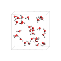
Run a short NVT equilibration at the low starting density.

from scm.plams import AMSNVTJob

nvt_low_density_job = AMSNVTJob(
    molecule=low_density_box,
    name="nvt_low_density_job",
    settings=reaxff_s,
    nsteps=3000,
    temperature=300,
    thermostat="Berendsen",
    tau=100,
    samplingfreq=500,
    timestep=0.5,
)
nvt_low_density_job.run();

[19.10|10:41:44] JOB nvt_low_density_job STARTED
[19.10|10:41:44] JOB nvt_low_density_job RUNNING
[19.10|10:41:48] JOB nvt_low_density_job FINISHED
[19.10|10:41:48] JOB nvt_low_density_job SUCCESSFUL

Use a regular AMSMDJob with a deformation toward a target density of 1.0 g/cm^3. This replaces the dedicated scan job while keeping the intermediate density-ramp stage explicit in the workflow.

from scm.inputs import AMS
from scm.plams import AMSMDJob

scan_density_settings = AMS()
scan_density_settings.MolecularDynamics.Deformation = [
    {"StartStep": 1, "StopStep": 6000, "TargetDensity": 1.0}
]

scan_density_job = AMSMDJob.restart_from(
    nvt_low_density_job,
    name="scan_density_job",
    settings=scan_density_settings,
    nsteps=6000,
    samplingfreq=100,
    temperature=300,
    thermostat="Berendsen",
    tau=100,
    timestep=0.5,
)
scan_density_job.run();

[19.10|10:41:48] JOB scan_density_job STARTED
[19.10|10:41:48] JOB scan_density_job RUNNING
[19.10|10:42:01] JOB scan_density_job FINISHED
[19.10|10:42:01] JOB scan_density_job SUCCESSFUL

import matplotlib.pyplot as plt
import numpy as np
from scm.base import Units


def plot_density(job, title=None, window: int = None):
    time = job.results.get_history_property("Time", "MDHistory")
    density = np.array(job.results.get_history_property("Density", "MDHistory"))
    density *= Units.conversion_factor("au", "kg") / Units.conversion_factor("bohr", "m") ** 3
    fig, ax = plt.subplots(figsize=(5, 3))
    ax.plot(time, density)
    ax.set_xlabel("Time (fs)")
    ax.set_ylabel("Density (kg/m^3)")
    ax.set_title(title or job.name + " Density")
    return ax


ax = plot_density(scan_density_job)
ax;

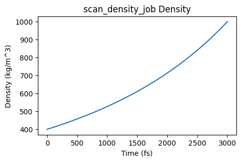
Continue with an NPT simulation from the final frame of the density-scan job.

from scm.plams import AMSNPTJob

npt_equilibration = AMSNPTJob.restart_from(
    scan_density_job,
    name="npt_equilibration",
    nsteps=20000,
    temperature=300,
    thermostat="Berendsen",
    tau=100,
    barostat="Berendsen",
    equal="XYZ",
    pressure=1e5,
    barostat_tau=1000,
)

npt_equilibration.run();

[19.10|10:42:01] JOB npt_equilibration STARTED
[19.10|10:42:01] JOB npt_equilibration RUNNING
[19.10|10:43:01] JOB npt_equilibration FINISHED
[19.10|10:43:01] JOB npt_equilibration SUCCESSFUL

ax = plot_density(npt_equilibration)
ax;

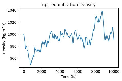
Extract a representative frame from the equilibrated part of the NPT trajectory. For production work, the simulation should generally be much longer before trusting the density.

from scm.plams import view

equilibrated_box = npt_equilibration.results.get_equilibrated_system()
print("Density: {:.2f} kg/m^3".format(equilibrated_box.density()))
equilibrated_box.write_xyz("water_equilibrated_box.xyz")
view(equilibrated_box, height=200, width=200, direction="tilt_z")

Density: 0.60 kg/m^3

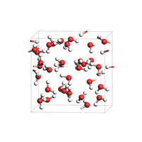
Note: get_equilibrated_system() is only available for the AMSNPTJob class and by default gets a structure from the last third of the simulation with a density that is close to the average during that segment.

This is different from get_main_system() which returns the final frame.

Python Script¶

#!/usr/bin/env python
# coding: utf-8

# ## ReaxFF density equilibration
# 
# Estimate the density predicted by ReaxFF for liquid water by starting from a low-density box, running a short NVT equilibration, using a deformation-based MD scan toward a target density, and then continuing with an NPT simulation. The example shows how to inspect the density trace and extract a representative equilibrated structure.
# 

# ReaxFF parallelizes with both MPI and OpenMP. To keep this example simple and reproducible, the run is configured in serial by setting ``nproc=1`` and ``OMP_NUM_THREADS=1``.
# 

from scm.inputs import AMS, ReaxFF
from scm.plams import Settings

reaxff_s = Settings()
reaxff_s.input = AMS(Engine=ReaxFF(ForceField="Water2017.ff"))
reaxff_s.runscript.nproc = 1
reaxff_s.runscript.preamble_lines = ["export OMP_NUM_THREADS=1"]


# Start from a deliberately loose liquid box so the short NVT run can relax the molecular arrangement before the density scan and barostat are switched on.
# 

from scm.base import ChemicalSystem
from scm.plams import packmol, preoptimize, view

low_density_box = packmol(ChemicalSystem.from_smiles("O"), n_molecules=32, region_names="water", density=0.4)
low_density_box = preoptimize(low_density_box, maxiterations=50)
view(low_density_box, height=200, width=200, direction="tilt_z", picture_path="picture1.png")


# Run a short NVT equilibration at the low starting density.
# 

from scm.plams import AMSNVTJob

nvt_low_density_job = AMSNVTJob(
    molecule=low_density_box,
    name="nvt_low_density_job",
    settings=reaxff_s,
    nsteps=3000,
    temperature=300,
    thermostat="Berendsen",
    tau=100,
    samplingfreq=500,
    timestep=0.5,
)
nvt_low_density_job.run();


# Use a regular ``AMSMDJob`` with a deformation toward a target density of ``1.0 g/cm^3``. This replaces the dedicated scan job while keeping the intermediate density-ramp stage explicit in the workflow.
# 

from scm.inputs import AMS
from scm.plams import AMSMDJob

scan_density_settings = AMS()
scan_density_settings.MolecularDynamics.Deformation = [
    {"StartStep": 1, "StopStep": 6000, "TargetDensity": 1.0}
]

scan_density_job = AMSMDJob.restart_from(
    nvt_low_density_job,
    name="scan_density_job",
    settings=scan_density_settings,
    nsteps=6000,
    samplingfreq=100,
    temperature=300,
    thermostat="Berendsen",
    tau=100,
    timestep=0.5,
)
scan_density_job.run();


import matplotlib.pyplot as plt
import numpy as np
from scm.base import Units


def plot_density(job, title=None, window: int = None):
    time = job.results.get_history_property("Time", "MDHistory")
    density = np.array(job.results.get_history_property("Density", "MDHistory"))
    density *= Units.conversion_factor("au", "kg") / Units.conversion_factor("bohr", "m") ** 3
    fig, ax = plt.subplots(figsize=(5, 3))
    ax.plot(time, density)
    ax.set_xlabel("Time (fs)")
    ax.set_ylabel("Density (kg/m^3)")
    ax.set_title(title or job.name + " Density")
    return ax


ax = plot_density(scan_density_job)
ax;
ax.figure.savefig("picture2.png")


# Continue with an NPT simulation from the final frame of the density-scan job.
# 

from scm.plams import AMSNPTJob

npt_equilibration = AMSNPTJob.restart_from(
    scan_density_job,
    name="npt_equilibration",
    nsteps=20000,
    temperature=300,
    thermostat="Berendsen",
    tau=100,
    barostat="Berendsen",
    equal="XYZ",
    pressure=1e5,
    barostat_tau=1000,
)

npt_equilibration.run();


ax = plot_density(npt_equilibration)
ax;
ax.figure.savefig("picture3.png")


# Extract a representative frame from the equilibrated part of the NPT trajectory. For production work, the simulation should generally be much longer before trusting the density.
# 

from scm.plams import view

equilibrated_box = npt_equilibration.results.get_equilibrated_system()
print("Density: {:.2f} kg/m^3".format(equilibrated_box.density()))
equilibrated_box.write_xyz("water_equilibrated_box.xyz")
view(equilibrated_box, height=200, width=200, direction="tilt_z", picture_path="picture4.png")


# Note: `get_equilibrated_system()` is only available for the AMSNPTJob class and by default gets a structure from the last third of the simulation with a density that is close to the average during that segment.
# 
# This is different from `get_main_system()` which returns the final frame.

ReaxFF Density Equilibration¶

ReaxFF density equilibration¶

See also¶

Related examples¶

Related tutorials¶

Related documentation¶

Python Script¶