Basic MD Trajectory Analysis with PLAMS

Molecular Dynamics Analysis Trajectory analysis

This example shows how to calculate several standard trajectory-analysis quantities from molecular dynamics:

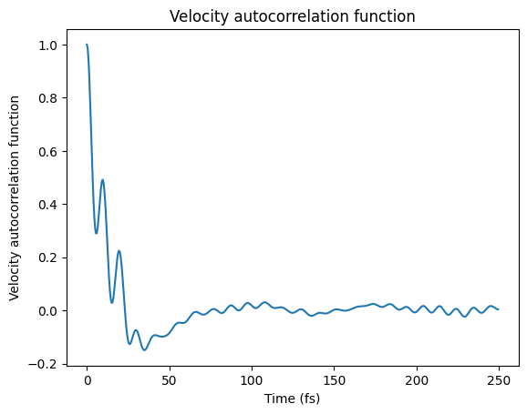
• the velocity autocorrelation function (VACF)

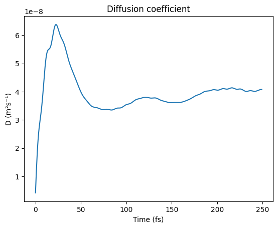
• the diffusion coefficient from the integral of the VACF

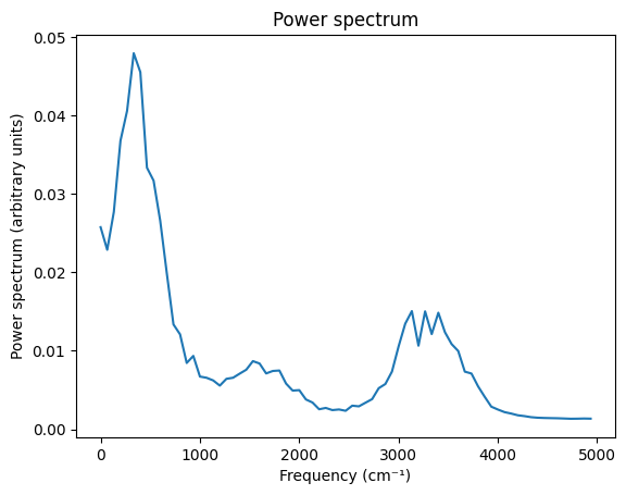
• the power spectrum from the Fourier transform of the VACF

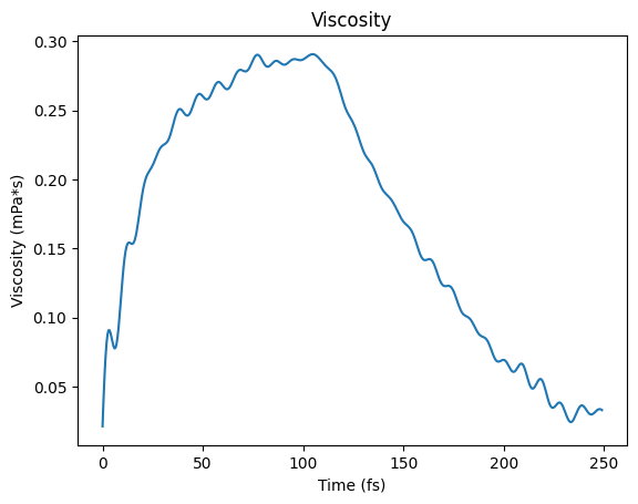
• the viscosity from the Green-Kubo relation using the off-diagonal pressure-tensor autocorrelation function

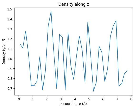
• the density profile along the z axis

The example focuses on the mechanics of extracting these quantities. For production simulations, the trajectories must be much longer and the analysis must be checked for convergence. For a broader molecular-dynamics workflow example, see also Molecular Dynamics with Python.

Downloads: Notebook | Script ?

Requires: AMS2027 or later

Related examples

• Molecular Dynamics with Python

• Viscosity from MD with the Green-Kubo Formalism

• PLUMED Biasing in AMS Molecular Dynamics

• Automated Transition-State Workflow for a Diels-Alder Addition

• Building Packed Systems with Packmol

Related tutorials

• Viscosity of benzene tutorial

Related documentation

• Trajectory analysis utilities

• Molecular Dynamics task

Initial Imports

import os
import numpy as np
import matplotlib.pyplot as plt
from scm.base import ChemicalSystem
from scm.inputs import AMS, ReaxFF
from scm.plams import packmol, Settings, AMSJob, view

Run Simple MD Simulation of Water

Run a short MD simulation of 16 water molecules in a box.

mol = packmol(ChemicalSystem.from_smiles("O"), n_molecules=16, density=1.0)
s = Settings()
s.input = AMS(Task="MolecularDynamics")
s.input.Engine = ReaxFF(ForceField="Water2017.ff")
s.input.MolecularDynamics.CalcPressure = True
s.input.MolecularDynamics.InitialVelocities.Temperature = 300
s.input.MolecularDynamics.Trajectory.SamplingFreq = 1
s.input.MolecularDynamics.TimeStep = 0.5
s.input.MolecularDynamics.NSteps = 2000
s.runscript.nproc = 1
os.environ["OMP_NUM_THREADS"] = "1"
job = AMSJob(settings=s, molecule=mol, name="md")
job.run();

[19.10|12:12:32] JOB md STARTED
[19.10|12:12:32] JOB md RUNNING
[19.10|12:12:37] JOB md FINISHED
[19.10|12:12:38] JOB md SUCCESSFUL

view(mol, direction="tilt_z", width=300, height=300, padding=-1)

Or alternatively, load a previously run MD job:

# job = AMSJob.load_external('/path/to/ams.rkf')
results = job.results

Velocity Autocorrelation Function

times, vacf = results.get_velocity_acf(start_fs=0, max_dt_fs=250, normalize=False)
normalized_vacf = vacf / vacf[0]

A = np.stack((times, normalized_vacf), axis=1)
np.savetxt("plams_vacf.txt", A, header="Time(fs) VACF")

fig, ax = plt.subplots()
ax.plot(times, normalized_vacf)
ax.set_xlabel("Time (fs)")
ax.set_ylabel("Velocity autocorrelation function")
ax.set_title("Velocity autocorrelation function")
ax;

Diffusion Coefficient

t_D, D = results.get_diffusion_coefficient_from_velocity_acf(times, vacf)

A = np.stack((t_D, D), axis=1)
np.savetxt("plams_vacf_D.txt", A, header="time(fs) D(m^2*s^-1)")

fig, ax = plt.subplots()
ax.plot(t_D, D)
ax.set_xlabel("Time (fs)")
ax.set_ylabel("D (m²s⁻¹)")
ax.set_title("Diffusion coefficient")
ax;

Power Spectrum

freq, intensities = results.get_power_spectrum(times, vacf, number_of_points=1000)

A = np.stack((freq, intensities), axis=1)
np.savetxt("plams_power_spectrum.txt", A, header="Frequency(cm^-1) PowerSpectrum")

fig, ax = plt.subplots()

ax.plot(freq, intensities)
ax.set_xlabel("Frequency (cm⁻¹)")
ax.set_ylabel("Power spectrum (arbitrary units)")
ax.set_title("Power spectrum")
ax;

Green-Kubo Viscosity

t, viscosity = results.get_green_kubo_viscosity(
    start_fs=0, max_dt_fs=250
)  # do not do this for NPT simulations

A = np.stack((t, viscosity), axis=1)
np.savetxt("plams_green_kubo_viscosity.txt", A, header="Time(fs) Viscosity(mPa*s)")

fig, ax = plt.subplots()

ax.plot(t, viscosity)
ax.set_xlabel("Time (fs)")
ax.set_ylabel("Viscosity (mPa*s)")
ax.set_title("Viscosity")
ax;

Density Along Axis

z, density = results.get_density_along_axis(
    axis="z", density_type="mass", bin_width=0.2, atom_indices=None
)

A = np.stack((z, density), axis=1)
np.savetxt("plams_density_along_z.txt", A, header="z(angstrom) density(g/cm^3)")

fig, ax = plt.subplots()

ax.plot(z, density)
ax.set_xlabel("z coordinate (Å)")
ax.set_ylabel("Density (g/cm³)")
ax.set_title("Density along z")
ax;

See also

Related examples

• Molecular Dynamics with Python

• Viscosity from MD with the Green-Kubo Formalism

• PLUMED Biasing in AMS Molecular Dynamics

• Automated Transition-State Workflow for a Diels-Alder Addition

• Building Packed Systems with Packmol

Related tutorials

• Viscosity of benzene tutorial

Related documentation

• Trajectory analysis utilities

• Molecular Dynamics task

Python Script

#!/usr/bin/env python
# coding: utf-8

# ## Initial Imports

import os
import numpy as np
import matplotlib.pyplot as plt
from scm.base import ChemicalSystem
from scm.inputs import AMS, ReaxFF
from scm.plams import packmol, Settings, AMSJob, view


# ## Run Simple MD Simulation of Water

# Run a short MD simulation of 16 water molecules in a box.

mol = packmol(ChemicalSystem.from_smiles("O"), n_molecules=16, density=1.0)
s = Settings()
s.input = AMS(Task="MolecularDynamics")
s.input.Engine = ReaxFF(ForceField="Water2017.ff")
s.input.MolecularDynamics.CalcPressure = True
s.input.MolecularDynamics.InitialVelocities.Temperature = 300
s.input.MolecularDynamics.Trajectory.SamplingFreq = 1
s.input.MolecularDynamics.TimeStep = 0.5
s.input.MolecularDynamics.NSteps = 2000
s.runscript.nproc = 1
os.environ["OMP_NUM_THREADS"] = "1"
job = AMSJob(settings=s, molecule=mol, name="md")
job.run();


view(mol, direction="tilt_z", width=300, height=300, padding=-1, picture_path="picture1.png")


# Or alternatively, load a previously run MD job:

# job = AMSJob.load_external('/path/to/ams.rkf')
results = job.results


# ## Velocity Autocorrelation Function

times, vacf = results.get_velocity_acf(start_fs=0, max_dt_fs=250, normalize=False)
normalized_vacf = vacf / vacf[0]

A = np.stack((times, normalized_vacf), axis=1)
np.savetxt("plams_vacf.txt", A, header="Time(fs) VACF")

fig, ax = plt.subplots()
ax.plot(times, normalized_vacf)
ax.set_xlabel("Time (fs)")
ax.set_ylabel("Velocity autocorrelation function")
ax.set_title("Velocity autocorrelation function")
ax;
ax.figure.savefig("picture2.png")


# ## Diffusion Coefficient

t_D, D = results.get_diffusion_coefficient_from_velocity_acf(times, vacf)

A = np.stack((t_D, D), axis=1)
np.savetxt("plams_vacf_D.txt", A, header="time(fs) D(m^2*s^-1)")

fig, ax = plt.subplots()
ax.plot(t_D, D)
ax.set_xlabel("Time (fs)")
ax.set_ylabel("D (m²s⁻¹)")
ax.set_title("Diffusion coefficient")
ax;
ax.figure.savefig("picture3.png")


# ## Power Spectrum

freq, intensities = results.get_power_spectrum(times, vacf, number_of_points=1000)

A = np.stack((freq, intensities), axis=1)
np.savetxt("plams_power_spectrum.txt", A, header="Frequency(cm^-1) PowerSpectrum")

fig, ax = plt.subplots()

ax.plot(freq, intensities)
ax.set_xlabel("Frequency (cm⁻¹)")
ax.set_ylabel("Power spectrum (arbitrary units)")
ax.set_title("Power spectrum")
ax;
ax.figure.savefig("picture4.png")


# ## Green-Kubo Viscosity 

t, viscosity = results.get_green_kubo_viscosity(
    start_fs=0, max_dt_fs=250
)  # do not do this for NPT simulations

A = np.stack((t, viscosity), axis=1)
np.savetxt("plams_green_kubo_viscosity.txt", A, header="Time(fs) Viscosity(mPa*s)")

fig, ax = plt.subplots()

ax.plot(t, viscosity)
ax.set_xlabel("Time (fs)")
ax.set_ylabel("Viscosity (mPa*s)")
ax.set_title("Viscosity")
ax;
ax.figure.savefig("picture5.png")


# ## Density Along Axis

z, density = results.get_density_along_axis(
    axis="z", density_type="mass", bin_width=0.2, atom_indices=None
)

A = np.stack((z, density), axis=1)
np.savetxt("plams_density_along_z.txt", A, header="z(angstrom) density(g/cm^3)")

fig, ax = plt.subplots()

ax.plot(z, density)
ax.set_xlabel("z coordinate (Å)")
ax.set_ylabel("Density (g/cm³)")
ax.set_title("Density along z")
ax;
ax.figure.savefig("picture6.png")