Benchmarking ML Potentials for Hydrocarbon Isomerization Energies
Compare several ML potentials on hydrocarbon isomerization reaction energies and inspect how closely they reproduce the reference ordering and energy differences.
Benchmarking Hydrocarbon Isomerization Energies
This benchmark aims to evaluate the accuracy of a range of machine learning potentials included in AMS, using the ISOC7 dataset from the paper: A.Karton and E.Semidalas, “Benchmarking Isomerization Energies for C5–C7 Hydrocarbons: The ISOC7 Database,” J. of Comp. Chem. 47(2) (2026): e70296, https://doi.org/10.1002/jcc.70296.
The ISOC7 dataset contains a diverse range of hydrocarbons from simple alkanes to highly strained systems featuring tetrahedrane units, as well as alkanes, alkenes, alkynes, and cyclic compounds. It has reference data to CCSD(T)/CBS level of accuracy and therefore provides a good benchmark for evaluating the accuracy of ML potentials for small organic systems.
Extract Reference ISOC7 Database
We first extract the ISOC7 database:
import os
import tarfile
from pathlib import Path

isoc7_tar = Path(os.environ["AMSHOME"]) / "atomicdata" / "Benchmarks" / "ISOC7.tar.gz"
isoc7 = Path("./ISOC7")

if not isoc7.exists():
    with tarfile.open(isoc7_tar, "r:gz") as tar:
        tar.extractall(path=Path.cwd())
Load XYZ Data
Then we load all the xyz files as PLAMS molecules:
import scm.plams as plams

molecules = plams.read_molecules(isoc7, formats=["xyz"])
We can see the number of loaded structures:
print(f"Number of loaded structures: {len(molecules)}")
Number of loaded structures: 1308
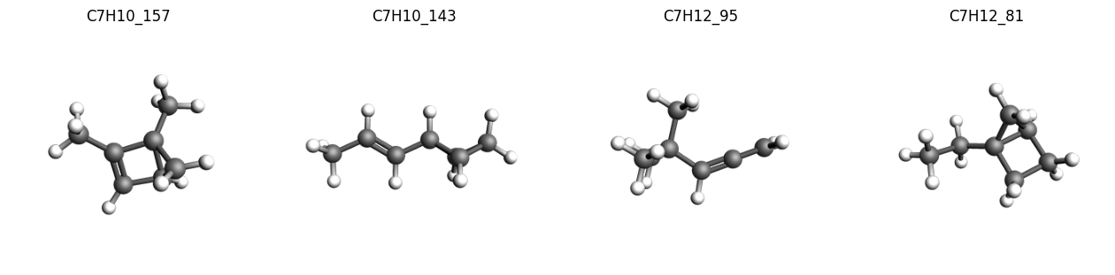
And view a selection of them, with their corresponding unique id:
imgs = {
    k: plams.view(v, width=300, height=300, guess_bonds=True)
    for k, v in list(molecules.items())[:4]
}

plams.plot_image_grid(imgs, rows=1);
Load Reference Data
Next we load the reference CCSD(T)/CBS energies from the benchmark:
import pandas as pd

reference_data = pd.read_csv(
    isoc7 / "ISOC7_W1-F12_Ref_Values.csv",
    usecols=[
        "reaction_name",
        "species1",
        "species2",
        "W1-F12_isomerization_energy (CCSD(T)/CBS, kcal/mol)",
    ],
)

reference_data
| reaction_name | species1 | species2 | W1-F12_isomerization_energy (CCSD(T)/CBS, kcal/mol) | |
|---|---|---|---|---|
| 0 | ISO_1 | C5H6_20 | C5H6_1 | 91.439 |
| 1 | ISO_2 | C5H6_20 | C5H6_2 | 90.146 |
| 2 | ISO_3 | C5H6_20 | C5H6_3 | 69.361 |
| 3 | ISO_4 | C5H6_20 | C5H6_4 | 61.970 |
| 4 | ISO_5 | C5H6_20 | C5H6_5 | 56.739 |
| ... | ... | ... | ... | ... |
| 1292 | ISO_1293 | C7H14_60 | C7H14_55 | 8.228 |
| 1293 | ISO_1294 | C7H14_60 | C7H14_56 | 6.718 |
| 1294 | ISO_1295 | C7H14_60 | C7H14_57 | 5.015 |
| 1295 | ISO_1296 | C7H14_60 | C7H14_58 | 4.639 |
| 1296 | ISO_1297 | C7H14_60 | C7H14_59 | 4.495 |
1297 rows × 4 columns
Set up Data Sets with ParAMS
To run our benchmark, we are going to user ParAMS. First we set up the JobCollection. This contains the information on the input structures.
import scm.params as params

results_importer = params.ResultsImporter(settings={"units": {"energy": "kcal/mol"}})
for k, v in molecules.items():
    jce = params.JCEntry()
    jce.settings.input.AMS.Task = "SinglePoint"
    jce.molecule = v
    jce.metadata["Source"] = "https://doi.org/10.1002/jcc.70296"
    results_importer.job_collection.add_entry(k, jce)
print(results_importer.job_collection.from_jobids(["C5H10_1"]))
---
dtype: JobCollection
version: '2026.102'
---
ID: 'C5H10_1'
ReferenceEngineID: None
AMSInput: |
   Task SinglePoint
   System
     Atoms
                 C      -2.0912640000       0.3020780000       0.0337330000
                 H      -1.8884470000       1.3092600000      -0.3363480000
                 H      -2.9862710000      -0.0691500000      -0.4691390000
                 H      -2.3168350000       0.3813300000       1.0998540000
                 C      -0.8950030000      -0.6171310000      -0.2050890000
                 H      -1.1307500000      -1.6274460000       0.1449640000
                 H      -0.7058150000      -0.7029420000      -1.2800580000
                 C       0.3616680000      -0.1305570000       0.4747630000
                 H       0.2826960000      -0.0502440000       1.5542310000
                 C       1.7140390000      -0.5126740000      -0.0538700000
                 H       1.7487570000      -1.1235900000      -0.9469660000
                 H       2.5092940000      -0.7118750000       0.6517470000
                 C       1.2230000000       0.9054910000      -0.1923400000
                 H       1.6860140000       1.6700050000       0.4167400000
                 H       0.9267080000       1.2414110000      -1.1782100000
     End
   End
Source: https://doi.org/10.1002/jcc.70296
...
Next we set up the dataset containing the information on each isomerization reaction and the reference energy:
ha_to_kcal_mol = plams.Units.conversion_ratio("Ha", "kcal/mol")

for _, (s1, s2, ref_e) in reference_data[
    ["species1", "species2", "W1-F12_isomerization_energy (CCSD(T)/CBS, kcal/mol)"]
].iterrows():
    results_importer.data_set.add_entry(
        f"energy('{s2}')-energy('{s1}')",
        reference=ref_e,
        unit=("kcal/mol", ha_to_kcal_mol),
        metadata={
            "Source": "https://doi.org/10.1002/jcc.70296",
            "reference_method": "CCSD(T)/CBS",
        },
    )
print(results_importer.data_set.from_jobids(["C5H6_1", "C5H6_20"]))
---
dtype: DataSet
version: '2026.102'
---
Expression: energy('C5H6_1')-energy('C5H6_20')
Weight: 1.0
Sigma: 0.002
ReferenceValue: 91.439
Unit: kcal/mol, 627.5094737775374
Source: https://doi.org/10.1002/jcc.70296
reference_method: CCSD(T)/CBS
...
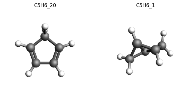
We can also visualize one of these isomerization reactions, for example the first one with a high isomerization energy:
imgs = {
    k: plams.view(molecules[k], width=300, height=300, guess_bonds=True)
    for k in ["C5H6_20", "C5H6_1"]
}

plams.plot_image_grid(imgs, rows=1);
Now we store the yaml files needed to run the ParAMS calculations:
results_importer.store("./isoc7_benchmark")
['./isoc7_benchmark/job_collection.yaml',
 './isoc7_benchmark/results_importer_settings.yaml',
 './isoc7_benchmark/training_set.yaml']
Note that the dataset can also be viewed using the ParAMS GUI:
# !params -gui ./isoc7_benchmark/job_collection.yaml
Run Benchmarks with ParAMS
Now we set up a benchmark job for each ML model of interest, and run them. We include all models suitable for small organic molecules, as well as some trained on materials/other domains for comparison.
models = [
    "AIMNet2-B973c",
    "AIMNet2-wB97MD3",
    "ANI-1ccx",
    "ANI-1x",
    "ANI-2x",
    "eSEN-S-Con-OMol",
    "M3GNet-UP-2022",
    "MACE-MPA-0",
    "UMA-S-1.2-ODAC",
    "UMA-S-1.2-OMat",
    "UMA-S-1.2-OMol",
]
jobs = {}

for model in models:
    job = params.ParAMSJob.from_yaml("./isoc7_benchmark", name=f"benchmark_{model}")
    job.settings.runscript.nproc = 1
    job.settings.runscript.preamble_lines = ["export OMP_NUM_THREADS=1"]
    job.settings.input.parallellevels.jobs = 1
    job.settings.input.mlpotential.model = model
    job.settings.input.task = "SinglePoint"
    jobs[model] = job
for job in jobs.values():
    job.run()
    job.ok()
[17.04|11:24:25] JOB benchmark_AIMNet2-B973c STARTED
[17.04|11:24:25] JOB benchmark_AIMNet2-B973c RUNNING
[17.04|11:24:54] JOB benchmark_AIMNet2-B973c FINISHED
[17.04|11:24:54] JOB benchmark_AIMNet2-B973c SUCCESSFUL
[17.04|11:24:54] JOB benchmark_AIMNet2-wB97MD3 STARTED
[17.04|11:24:54] JOB benchmark_AIMNet2-wB97MD3 RUNNING
[17.04|11:25:22] JOB benchmark_AIMNet2-wB97MD3 FINISHED
[17.04|11:25:22] JOB benchmark_AIMNet2-wB97MD3 SUCCESSFUL
[17.04|11:25:22] JOB benchmark_ANI-1ccx STARTED
[17.04|11:25:22] JOB benchmark_ANI-1ccx RUNNING
[17.04|11:25:35] JOB benchmark_ANI-1ccx FINISHED
[17.04|11:25:35] JOB benchmark_ANI-1ccx SUCCESSFUL
[17.04|11:25:35] JOB benchmark_ANI-1x STARTED
[17.04|11:25:35] JOB benchmark_ANI-1x RUNNING
[17.04|11:25:48] JOB benchmark_ANI-1x FINISHED
[17.04|11:25:48] JOB benchmark_ANI-1x SUCCESSFUL
[17.04|11:25:48] JOB benchmark_ANI-2x STARTED
... output trimmed ....
[17.04|11:27:55] JOB benchmark_M3GNet-UP-2022 SUCCESSFUL
[17.04|11:27:55] JOB benchmark_MACE-MPA-0 STARTED
[17.04|11:27:55] JOB benchmark_MACE-MPA-0 RUNNING
[17.04|11:28:59] JOB benchmark_MACE-MPA-0 FINISHED
[17.04|11:28:59] JOB benchmark_MACE-MPA-0 SUCCESSFUL
[17.04|11:28:59] JOB benchmark_UMA-S-1.2-ODAC STARTED
[17.04|11:28:59] JOB benchmark_UMA-S-1.2-ODAC RUNNING
[17.04|11:31:28] JOB benchmark_UMA-S-1.2-ODAC FINISHED
[17.04|11:31:29] JOB benchmark_UMA-S-1.2-ODAC SUCCESSFUL
[17.04|11:31:29] JOB benchmark_UMA-S-1.2-OMat STARTED
[17.04|11:31:29] JOB benchmark_UMA-S-1.2-OMat RUNNING
[17.04|11:33:54] JOB benchmark_UMA-S-1.2-OMat FINISHED
[17.04|11:33:54] JOB benchmark_UMA-S-1.2-OMat SUCCESSFUL
[17.04|11:33:54] JOB benchmark_UMA-S-1.2-OMol STARTED
[17.04|11:33:54] JOB benchmark_UMA-S-1.2-OMol RUNNING
[17.04|11:36:16] JOB benchmark_UMA-S-1.2-OMol FINISHED
[17.04|11:36:16] JOB benchmark_UMA-S-1.2-OMol SUCCESSFUL
Each completed job now has results for the errors between the model calculations and the reference. For example, with AIMNet2-wB97MD3:
print("\n".join(str(jobs["AIMNet2-wB97MD3"].results.get_data_set_evaluator()).split("\n")[:20]))
Group/Expression            N        MAE          RMSE*        Unit*          Weight     Loss*        Contribution[%]
---------------------------------------------------------------------------------------------------------------------
Total                       1297     1.28848      +1.60312     kcal/mol       1297.000   833315816.952 100.00     Total

   energy                   1297     1.28848      +1.60312     kcal/mol       1297.000   833315816.952 100.00     Extractor
      C7H8_51-C7H8_320      1        7.03500      -7.03500     kcal/mol       1.000      12372796.117 1.48       Expression
      C7H8_3-C7H8_320       1        6.84835      -6.84835     kcal/mol       1.000      11724976.294 1.41       Expression
      C6H6_2-C6H6_56        1        6.80974      -6.80974     kcal/mol       1.000      11593141.526 1.39       Expression
      C7H8_117-C7H8_320     1        6.56349      -6.56349     kcal/mol       1.000      10769839.645 1.29       Expression
      C7H8_79-C7H8_320      1        6.54360      -6.54360     kcal/mol       1.000      10704671.280 1.28       Expression
      C6H6_21-C6H6_56       1        6.35571      -6.35571     kcal/mol       1.000      10098752.565 1.21       Expression
      C7H8_10-C7H8_320      1        6.00152      -6.00152     kcal/mol       1.000      9004556.137  1.08       Expression
      C7H8_256-C7H8_320     1        5.79461      -5.79461     kcal/mol       1.000      8394388.810  1.01       Expression
      C7H8_9-C7H8_320       1        5.52882      -5.52882     kcal/mol       1.000      7641966.144  0.92       Expression
      C7H8_66-C7H8_320      1        5.14151      -5.14151     kcal/mol       1.000      6608776.360  0.79       Expression
      C7H8_4-C7H8_320       1        5.13745      -5.13745     kcal/mol       1.000      6598337.286  0.79       Expression
      C7H8_5-C7H8_320       1        4.50864      -4.50864     kcal/mol       1.000      5081948.943  0.61       Expression
      C7H8_44-C7H8_320      1        4.41894      -4.41894     kcal/mol       1.000      4881765.891  0.59       Expression
      C7H8_266-C7H8_320     1        4.04698      -4.04698     kcal/mol       1.000      4094507.700  0.49       Expression
      C7H10_35-C7H10_396    1        3.99482      +3.99482     kcal/mol       1.000      3989642.301  0.48       Expression
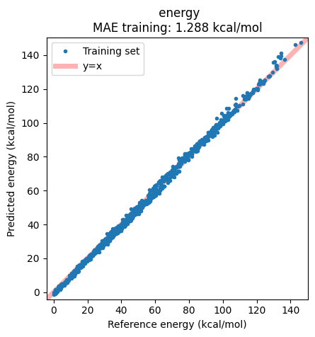
Results can alternatively be displayed in a correlation plot of the reference vs. predicted energies:
ax = jobs["AIMNet2-wB97MD3"].results.plot_simple_correlation("energy", validation_set=False)
ax;
Note that all these can also again be viewed in the ParAMS GUI:
# !params -gui ./plams_workdir/benchmark_AIMNet2-wB97MD3/results
Evaluating Benchmark Results
To evaluate the results, we extract the Mean Absolute Error (MAE) and Root Mean Squared Error (RMSE) from the job results:
results = pd.DataFrame({"Model": models})
results["MAE"] = [jobs[m].results.get_data_set_evaluator().results.mae for m in models]
results["RMSE"] = [jobs[m].results.get_data_set_evaluator().results.rmse for m in models]
results.sort_values(by="MAE", inplace=True)
results.rename(
    columns={
        "MAE": "MAE<sup>*</sup>",
        "RMSE": "RMSE<sup>*</sup>",
    },
    inplace=True,
)
results.style.hide(axis="index").background_gradient(
    subset=["MAE<sup>*</sup>", "RMSE<sup>*</sup>"], cmap="Blues", vmin=0, vmax=10
).format("{:.2f}", subset=["MAE<sup>*</sup>", "RMSE<sup>*</sup>"]).set_caption(
    "<br><span style='text-align:left;font-size:18px'>Benchmark Results for <a href='https://doi.org/10.1002/jcc.70296' target='_blank'>ISOC7 Dataset</a> Isomerization Energies</span>"
    "<br><span style='font-size:14px'><sup>*</sup> Reference method CCSD(T)/CBS, in kcal/mol</span>"
).set_table_styles(
    [
        {"selector": "th", "props": [("border-bottom", "2px solid black")]},
        {"selector": "th, td", "props": [("min-width", "100px")]},
        {"selector": "td", "props": [("border-bottom", "1px solid lightgray")]},
        {"selector": "table", "props": [("border-collapse", "collapse")]},
    ]
)
| Model | MAE* | RMSE* |
|---|---|---|
| eSEN-S-Con-OMol | 1.07 | 1.32 |
| UMA-S-1.2-OMol | 1.09 | 1.34 |
| AIMNet2-wB97MD3 | 1.29 | 1.60 |
| UMA-S-1.2-OMat | 2.88 | 3.62 |
| ANI-1ccx | 3.08 | 5.17 |
| AIMNet2-B973c | 4.16 | 4.96 |
| UMA-S-1.2-ODAC | 4.92 | 6.23 |
| ANI-1x | 5.15 | 6.65 |
| ANI-2x | 5.75 | 7.29 |
| M3GNet-UP-2022 | 7.82 | 10.09 |
| MACE-MPA-0 | 13.46 | 15.47 |
From these results, we see that eSEN-S-Con-OMol, UMA-S-1.2-OMol
and AIMNet2-wB97MD3 perform best, achieving the lowest errors
(eSEN-S-Con-OMol having MAE = 1.07 kcal/mol, RMSE = 1.32 kcal/mol).
We note that all of these are trained on datasets with ωB97M-D3(BJ) as
the reference method. In a broader context, the accuracy of these models
is therefore on a par with the best performing DFT functionals, at a
fraction of the computational cost.
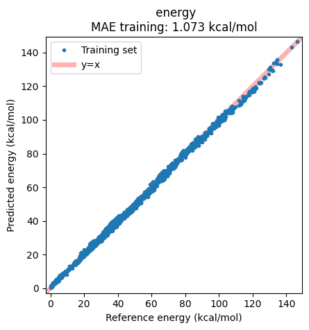
Plotting the correlation between reference and predicted energies shows the success of the model, with essentially no real outliers.
ax = jobs["eSEN-S-Con-OMol"].results.plot_simple_correlation("energy", validation_set=False)
ax;
Other models targeted at small molecules also perform well, including
ANI-1ccx and AIMNet2-B973c, with MAE < 5 kcal/mol.
The correlation plot shows, however, that in this case there are some structures which are not well captured by the model:
ax = jobs["ANI-1ccx"].results.plot_simple_correlation("energy", validation_set=False)
ax;
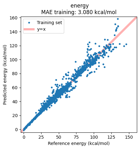
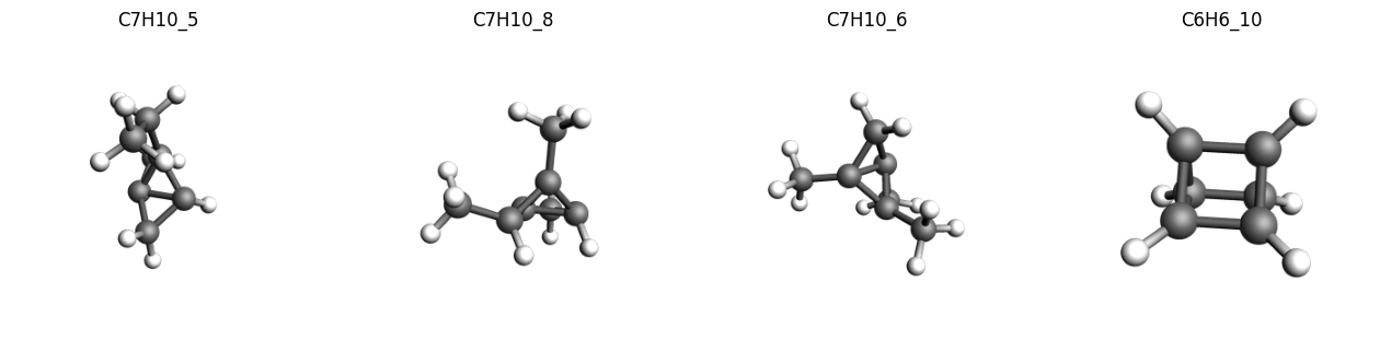
We can extract these outlier structures from the data and inspect them.
As noted in the original paper, we find many of the systems with a high deviations compared to the reference values contain a highly strained ring systems or tetrahedrane cores, which is also a common issue with many of the tested DFT functionals.
print("\n".join(str(jobs["ANI-1ccx"].results.get_data_set_evaluator()).split("\n")[:9]))
Group/Expression            N        MAE          RMSE*        Unit*          Weight     Loss*        Contribution[%]
---------------------------------------------------------------------------------------------------------------------
Total                       1297     3.07973      +5.17159     kcal/mol       1297.000   8672162574.204 100.00     Total

   energy                   1297     3.07973      +5.17159     kcal/mol       1297.000   8672162574.204 100.00     Extractor
      C7H10_5-C7H10_396     1        31.12503     -31.12503    kcal/mol       1.000      242191863.432 2.79       Expression
      C7H10_8-C7H10_396     1        30.82095     -30.82095    kcal/mol       1.000      237482804.138 2.74       Expression
      C7H10_6-C7H10_396     1        26.50819     -26.50819    kcal/mol       1.000      175671019.698 2.03       Expression
      C6H6_10-C6H6_56       1        25.57246     +25.57246    kcal/mol       1.000      163487616.549 1.89       Expression
imgs = {
    k: plams.view(molecules[k], width=300, height=300, guess_bonds=True)
    for k in ["C7H10_5", "C7H10_8", "C7H10_6", "C6H6_10"]
}

plams.plot_image_grid(imgs, rows=1);
Finally, we find that, as expected, the worst performers in this
benchmark are models trained primarily on materials data such as
M3GNet-UP-2022 and MACE-MPA-0, which are better suited to other
chemical domains.
See also
Python Script
#!/usr/bin/env python
# coding: utf-8

# ## Benchmarking Hydrocarbon Isomerization Energies

# This benchmark aims to evaluate the accuracy of a range of machine learning potentials included in AMS, using the ISOC7 dataset from the paper: A.Karton and E.Semidalas, “Benchmarking Isomerization Energies for C5–C7 Hydrocarbons: The ISOC7 Database,” J. of Comp. Chem. 47(2) (2026): e70296, https://doi.org/10.1002/jcc.70296.
#
# The ISOC7 dataset contains a diverse range of hydrocarbons from simple alkanes to highly strained systems featuring tetrahedrane units, as well as alkanes, alkenes, alkynes, and cyclic compounds. It has reference data to CCSD(T)/CBS level of accuracy and therefore provides a good benchmark for evaluating the accuracy of ML potentials for small organic systems.

# ### Extract Reference ISOC7 Database

# We first extract the ISOC7 database:

import os
import tarfile
from pathlib import Path

isoc7_tar = Path(os.environ["AMSHOME"]) / "atomicdata" / "Benchmarks" / "ISOC7.tar.gz"
isoc7 = Path("./ISOC7")

if not isoc7.exists():
    with tarfile.open(isoc7_tar, "r:gz") as tar:
        tar.extractall(path=Path.cwd())


# ### Load XYZ Data

# Then we load all the xyz files as PLAMS molecules:

import scm.plams as plams

molecules = plams.read_molecules(isoc7, formats=["xyz"])


# We can see the number of loaded structures:

print(f"Number of loaded structures: {len(molecules)}")


# And view a selection of them, with their corresponding unique id:

imgs = {k: plams.view(v, width=300, height=300, guess_bonds=True) for k, v in list(molecules.items())[:4]}

plams.plot_image_grid(imgs, rows=1, save_path="picture1.png")
# ### Load Reference Data

# Next we load the reference CCSD(T)/CBS energies from the benchmark:

import pandas as pd

reference_data = pd.read_csv(
    isoc7 / "ISOC7_W1-F12_Ref_Values.csv",
    usecols=[
        "reaction_name",
        "species1",
        "species2",
        "W1-F12_isomerization_energy (CCSD(T)/CBS, kcal/mol)",
    ],
)

reference_data


# ### Set up Data Sets with ParAMS

# To run our benchmark, we are going to user ParAMS. First we set up the JobCollection. This contains the information on the input structures.

import scm.params as params

results_importer = params.ResultsImporter(settings={"units": {"energy": "kcal/mol"}})


for k, v in molecules.items():
    jce = params.JCEntry()
    jce.settings.input.AMS.Task = "SinglePoint"
    jce.molecule = v
    jce.metadata["Source"] = "https://doi.org/10.1002/jcc.70296"
    results_importer.job_collection.add_entry(k, jce)


print(results_importer.job_collection.from_jobids(["C5H10_1"]))


# Next we set up the dataset containing the information on each isomerization reaction and the reference energy:

ha_to_kcal_mol = plams.Units.conversion_ratio("Ha", "kcal/mol")

for _, (s1, s2, ref_e) in reference_data[
    ["species1", "species2", "W1-F12_isomerization_energy (CCSD(T)/CBS, kcal/mol)"]
].iterrows():
    results_importer.data_set.add_entry(
        f"energy('{s2}')-energy('{s1}')",
        reference=ref_e,
        unit=("kcal/mol", ha_to_kcal_mol),
        metadata={
            "Source": "https://doi.org/10.1002/jcc.70296",
            "reference_method": "CCSD(T)/CBS",
        },
    )


print(results_importer.data_set.from_jobids(["C5H6_1", "C5H6_20"]))


# We can also visualize one of these isomerization reactions, for example the first one with a high isomerization energy:

imgs = {k: plams.view(molecules[k], width=300, height=300, guess_bonds=True) for k in ["C5H6_20", "C5H6_1"]}

plams.plot_image_grid(imgs, rows=1, save_path="picture2.png")
# Now we store the yaml files needed to run the ParAMS calculations:

results_importer.store("./isoc7_benchmark")


# Note that the dataset can also be viewed using the ParAMS GUI:

# !params -gui ./isoc7_benchmark/job_collection.yaml


# ### Run Benchmarks with ParAMS

# Now we set up a benchmark job for each ML model of interest, and run them. We include all models suitable for small organic molecules, as well as some trained on materials/other domains for comparison.

models = [
    "AIMNet2-B973c",
    "AIMNet2-wB97MD3",
    "ANI-1ccx",
    "ANI-1x",
    "ANI-2x",
    "eSEN-S-Con-OMol",
    "M3GNet-UP-2022",
    "MACE-MPA-0",
    "UMA-S-1.2-ODAC",
    "UMA-S-1.2-OMat",
    "UMA-S-1.2-OMol",
]


jobs = {}

for model in models:
    job = params.ParAMSJob.from_yaml("./isoc7_benchmark", name=f"benchmark_{model}")
    job.settings.runscript.nproc = 1
    job.settings.runscript.preamble_lines = ["export OMP_NUM_THREADS=1"]
    job.settings.input.parallellevels.jobs = 1
    job.settings.input.mlpotential.model = model
    job.settings.input.task = "SinglePoint"
    jobs[model] = job


for job in jobs.values():
    job.run()
    job.ok()


# Each completed job now has results for the errors between the model calculations and the reference. For example, with AIMNet2-wB97MD3:

print("\n".join(str(jobs["AIMNet2-wB97MD3"].results.get_data_set_evaluator()).split("\n")[:20]))


# Results can alternatively be displayed in a correlation plot of the reference vs. predicted energies:

ax = jobs["AIMNet2-wB97MD3"].results.plot_simple_correlation("energy", validation_set=False)
ax
ax.figure.savefig("picture3.png")


# Note that all these can also again be viewed in the ParAMS GUI:

# !params -gui ./plams_workdir/benchmark_AIMNet2-wB97MD3/results


# ## Evaluating Benchmark Results

# To evaluate the results, we extract the Mean Absolute Error (MAE) and Root Mean Squared Error (RMSE) from the job results:

results = pd.DataFrame({"Model": models})


results["MAE"] = [jobs[m].results.get_data_set_evaluator().results.mae for m in models]
results["RMSE"] = [jobs[m].results.get_data_set_evaluator().results.rmse for m in models]


results.sort_values(by="MAE", inplace=True)


results.rename(
    columns={
        "MAE": "MAE<sup>*</sup>",
        "RMSE": "RMSE<sup>*</sup>",
    },
    inplace=True,
)


results.style.hide(axis="index").background_gradient(
    subset=["MAE<sup>*</sup>", "RMSE<sup>*</sup>"], cmap="Blues", vmin=0, vmax=10
).format("{:.2f}", subset=["MAE<sup>*</sup>", "RMSE<sup>*</sup>"]).set_caption(
    "<br><span style='text-align:left;font-size:18px'>Benchmark Results for <a href='https://doi.org/10.1002/jcc.70296' target='_blank'>ISOC7 Dataset</a> Isomerization Energies</span>"
    "<br><span style='font-size:14px'><sup>*</sup> Reference method CCSD(T)/CBS, in kcal/mol</span>"
).set_table_styles(
    [
        {"selector": "th", "props": [("border-bottom", "2px solid black")]},
        {"selector": "th, td", "props": [("min-width", "100px")]},
        {"selector": "td", "props": [("border-bottom", "1px solid lightgray")]},
        {"selector": "table", "props": [("border-collapse", "collapse")]},
    ]
)


# From these results, we see that `eSEN-S-Con-OMol`, `UMA-S-1.2-OMol` and `AIMNet2-wB97MD3` perform best, achieving the lowest errors (`eSEN-S-Con-OMol` having MAE = 1.07 kcal/mol, RMSE = 1.32 kcal/mol). We note that all of these are trained on datasets with ωB97M-D3(BJ) as the reference method. In a broader context, the accuracy of these models is therefore on a par with the best performing DFT functionals, at a fraction of the computational cost.
#
# Plotting the correlation between reference and predicted energies shows the success of the model, with essentially no real outliers.

ax = jobs["eSEN-S-Con-OMol"].results.plot_simple_correlation("energy", validation_set=False)
ax
ax.figure.savefig("picture4.png")


# Other models targeted at small molecules also perform well, including `ANI-1ccx` and `AIMNet2-B973c`, with MAE < 5 kcal/mol.
#
# The correlation plot shows, however, that in this case there are some structures which are not well captured by the model:

ax = jobs["ANI-1ccx"].results.plot_simple_correlation("energy", validation_set=False)
ax
ax.figure.savefig("picture5.png")


# We can extract these outlier structures from the data and inspect them.
#
# As noted in the original paper, we find many of the systems with a high deviations compared to the reference values contain a highly strained ring systems or tetrahedrane cores, which is also a common issue with many of the tested DFT functionals.

print("\n".join(str(jobs["ANI-1ccx"].results.get_data_set_evaluator()).split("\n")[:9]))


imgs = {
    k: plams.view(molecules[k], width=300, height=300, guess_bonds=True)
    for k in ["C7H10_5", "C7H10_8", "C7H10_6", "C6H6_10"]
}

plams.plot_image_grid(imgs, rows=1, save_path="picture6.png")


# Finally, we find that, as expected, the worst performers in this benchmark are models trained primarily on materials data such as `M3GNet-UP-2022` and `MACE-MPA-0`, which are better suited to other chemical domains.