Active Learning: Liquid Water Properties¶

Train an active-learning M3GNet model for liquid water and validate it against diffusion, radial distribution functions, and density from molecular-dynamics simulations.

Downloads: Notebook | Script ?

Requires: AMS2026 or later

Required AMS Packages: m3gnet

../_images/active_learning_liquid_water_properties_67_0_f30c3b3f.png

When running active learning it’s usually a good idea to start off “simple” and make the system/structures gradually more complicated.

To train liquid water, we here

first train a potential at slightly above room temperature and 1.0 g/cm^3
continue with a second active learning loop where the density is explicitly scanned from a low to a high value

Initial imports¶

import scm.plams as plams
from scm.simple_active_learning import SimpleActiveLearningJob
import matplotlib.pyplot as plt
from scm.external_engines.core import interface_is_installed

assert interface_is_installed("m3gnet"), (
    "You must install the m3gnet backend before following this tutorial!"
)

plams.init()

PLAMS working folder: /path/to/plams_workdir.003

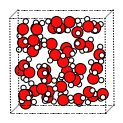
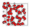
Create an initial water box¶

water = plams.from_smiles("O")
for at in water:
    at.properties = plams.Settings()
plams.plot_molecule(water)

box = plams.packmol(water, n_molecules=48, density=1.0)
plams.plot_molecule(box, rotation="-5x,5y,0z")

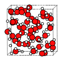
Let’s run a short MD simulation with M3GNet-UP-2022 to make the structure more realistic:

up_s = plams.Settings()
up_s.input.MLPotential.Model = "M3GNet-UP-2022"
up_s.runscript.nproc = 1  # always run AMS Driver in serial for MLPotential
up_md = plams.AMSNVTJob(
    molecule=box,
    settings=up_s,
    name="up_md",
    nsteps=1000,
    timestep=0.5,
    temperature=350,
)
up_md.run();

[22.02|09:51:37] JOB up_md STARTED
[22.02|09:51:37] JOB up_md RUNNING
[22.02|09:52:19] JOB up_md FINISHED
[22.02|09:52:20] JOB up_md SUCCESSFUL

<scm.plams.interfaces.adfsuite.ams.AMSResults at 0x7fccbdae5a90>

New structure:

starting_structure = up_md.results.get_main_molecule()
plams.plot_molecule(starting_structure, rotation="-5x,5y,0z")

Simple Active Learning setup¶

Reference engine settings¶

Here, we choose to train against ReaxFF Water-2017.ff, which gives a good water structure.

fast_ref_s = plams.Settings()
fast_ref_s.input.ReaxFF.ForceField = "Water2017.ff"
fast_ref_s.runscript.nproc = 1

slow_ref_s = plams.Settings()
slow_ref_s.input.QuantumESPRESSO.Pseudopotentials.Family = "SSSP-Efficiency"
slow_ref_s.input.QuantumESPRESSO.Pseudopotentials.Functional = "PBE"
slow_ref_s.input.QuantumESPRESSO.K_Points._h = "gamma"
slow_ref_s.input.QuantumESPRESSO.System = plams.Settings(
    input_dft="revpbe", ecutwfc=40, vdw_corr="Grimme-D3", dftd3_version=4
)

Change to slow_ref_s to train to revPBE-D3(BJ) instead:

ref_s = fast_ref_s.copy()

NVT molecular dynamics settings¶

nvt_md_s = plams.AMSNVTJob(
    nsteps=20000,
    timestep=0.5,
    temperature=(270, 350, 350),
    tau=100,
    thermostat="Berendsen",
).settings

ParAMS machine learning settings¶

ml_s = plams.Settings()
ml_s.input.ams.MachineLearning.Backend = "M3GNet"
ml_s.input.ams.MachineLearning.CommitteeSize = 1
ml_s.input.ams.MachineLearning.M3GNet.Model = "UniversalPotential"
ml_s.input.ams.MachineLearning.MaxEpochs = 200

Active learning settings¶

Liquid water is a “simple” homogeneous system, so we can expect the ML method to perform quite well. We therefore decrease the success criteria thresholds a bit compared to the default vvalues, to ensure that we get accurate results.

Since we will immediately continue with another active learning loop, we disable the “RerunSimulation” as we are not interested in the MD simulation per se.

al_s = plams.Settings()
al_s.input.ams.ActiveLearning.Steps.Type = "Geometric"
al_s.input.ams.ActiveLearning.Steps.Geometric.Start = 10
al_s.input.ams.ActiveLearning.Steps.Geometric.NumSteps = 8
al_s.input.ams.ActiveLearning.InitialReferenceData.Generate.M3GNetShortMD.Enabled = (
    "Yes"
)
al_s.input.ams.ActiveLearning.SuccessCriteria.Energy.Relative = 0.003
al_s.input.ams.ActiveLearning.SuccessCriteria.Forces.MaxDeviationForZeroForce = 0.35
al_s.input.ams.ActiveLearning.AtEnd.RerunSimulation = "No"

Complete job¶

settings = ref_s + nvt_md_s + ml_s + al_s
job = SimpleActiveLearningJob(
    settings=settings, molecule=starting_structure, name="sal"
)
print(job.get_input())

ActiveLearning
  AtEnd
    RerunSimulation False
  End
  InitialReferenceData
... output trimmed ....
         0.0000000000    11.2817834662     0.0000000000
         0.0000000000     0.0000000000    11.2817834662
  End
End

Run the simple active learning job¶

job.run(watch=True);

[22.02|10:12:07] JOB sal STARTED
[22.02|10:12:07] Renaming job sal to sal.002
[22.02|10:12:07] JOB sal.002 RUNNING
[22.02|10:12:09] Simple Active Learning 2024.101,  Nodes: 1, Procs: 1
[22.02|10:12:11] Composition of main system: H96O48
... output trimmed ....

[22.02|10:36:15] Active learning finished!
[22.02|10:36:15] Goodbye!
[22.02|10:36:15] JOB sal.002 FINISHED
[22.02|10:36:15] JOB sal.002 SUCCESSFUL





<scm.simple_active_learning.plams.simple_active_learning_job.SimpleActiveLearningResults at 0x7fccbe25c580>

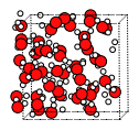
Validate trained model by RDF and MSD¶

Note: You should skip this part if you trained to DFT since the reference MD calculation will take a very long time!

mol = job.results.get_main_molecule()
plams.plot_molecule(mol, rotation="-5x,5y,0z")

retrained_model_settings = (
    job.results.get_params_job().results.get_production_engine_settings()
)
retrained_model_settings.runscript.nproc = 1

Equilibration and production MD settings¶

eq_md_settings = plams.AMSNVTJob(
    nsteps=8000,
    timestep=0.5,
    thermostat="Berendsen",
    tau=100,
    temperature=300,
    samplingfreq=100,
).settings

prod_md_settings = plams.AMSNVTJob(
    nsteps=50000,
    timestep=0.5,
    thermostat="NHC",
    tau=200,
    temperature=300,
    samplingfreq=100,
).settings

Retrained model equilibration¶

retrained_model_eq_md_job = plams.AMSJob(
    settings=eq_md_settings + retrained_model_settings,
    molecule=mol,
    name="retrained_model_eq_md_dens_1",
)
retrained_model_eq_md_job.run();

[22.02|13:39:24] JOB eq_md_dens_1 STARTED
[22.02|13:39:24] Renaming job eq_md_dens_1 to eq_md_dens_1.003
[22.02|13:39:24] JOB eq_md_dens_1.003 RUNNING
[22.02|13:42:58] JOB eq_md_dens_1.003 FINISHED
[22.02|13:42:58] JOB eq_md_dens_1.003 SUCCESSFUL

Retrained model production simulation¶

Let’s then run a production simulation from the final structure of the above equilibration MD using both the retrained model and the reference engine:

retrained_model_prod_md_job = plams.AMSJob(
    settings=prod_md_settings + retrained_model_settings,
    name="retrained_model_prod_md_dens_1",
    molecule=retrained_model_eq_md_job.results.get_main_molecule(),
)
retrained_model_prod_md_job.run();

[22.02|13:46:22] JOB retrained_model_prod_md_dens_1 STARTED
[22.02|13:46:22] Renaming job retrained_model_prod_md_dens_1 to retrained_model_prod_md_dens_1.005
[22.02|13:46:22] JOB retrained_model_prod_md_dens_1.005 RUNNING
[22.02|14:07:30] JOB retrained_model_prod_md_dens_1.005 FINISHED
[22.02|14:07:30] JOB retrained_model_prod_md_dens_1.005 SUCCESSFUL

Reference equilibration MD¶

reference_eq_md_job = plams.AMSJob(
    settings=eq_md_settings + ref_s,
    molecule=mol,
    name="reference_eq_md_dens_1",
)
reference_eq_md_job.run();

[22.02|14:08:55] JOB reference_eq_md_dens_1 STARTED
[22.02|14:08:55] JOB reference_eq_md_dens_1 RUNNING
[22.02|14:09:19] JOB reference_eq_md_dens_1 FINISHED
[22.02|14:09:19] JOB reference_eq_md_dens_1 SUCCESSFUL

Reference production MD¶

reference_prod_md_job = plams.AMSJob(
    settings=prod_md_settings + ref_s,
    name="reference_prod_md_dens_1",
    molecule=reference_eq_md_job.results.get_main_molecule(),
)
reference_prod_md_job.run();

[22.02|14:09:19] JOB reference_prod_md_dens_1 STARTED
[22.02|14:09:19] Renaming job reference_prod_md_dens_1 to reference_prod_md_dens_1.003
[22.02|14:09:19] JOB reference_prod_md_dens_1.003 RUNNING
[22.02|14:11:59] JOB reference_prod_md_dens_1.003 FINISHED
[22.02|14:11:59] JOB reference_prod_md_dens_1.003 SUCCESSFUL

Mean squared displacement (MSD) helper functions¶

For a detailed explanation of the MSD and RDF jobs, see the “Molecular dynamics with Python” tutorial

def get_msd_job(job: plams.AMSJob, symbol: str = "O"):
    atom_indices = [
        i
        for i, at in enumerate(job.results.get_main_molecule(), 1)
        if at.symbol == symbol
    ]

    msd_job = plams.AMSMSDJob(
        job,
        name="msd-" + job.name,
        atom_indices=atom_indices,  # indices start with 1 for the first atom
        max_correlation_time_fs=4000,  # max correlation time must be set before running the job
        start_time_fit_fs=2000,  # start_time_fit can also be changed later in the postanalysis
    )
    msd_job.run()

    return msd_job


def plot_msd(job, start_time_fit_fs=None):
    """job: an AMSMSDJob"""
    time, msd = job.results.get_msd()
    fit_result, fit_x, fit_y = job.results.get_linear_fit(
        start_time_fit_fs=start_time_fit_fs
    )
    # the diffusion coefficient can also be calculated as fit_result.slope/6 (ang^2/fs)
    diffusion_coefficient = job.results.get_diffusion_coefficient(
        start_time_fit_fs=start_time_fit_fs
    )  # m^2/s
    plt.figure(figsize=(5, 3))
    plt.plot(time, msd, label="MSD")
    plt.plot(
        fit_x, fit_y, label="Linear fit slope={:.5f} ang^2/fs".format(fit_result.slope)
    )
    plt.legend()
    plt.xlabel("Correlation time (fs)")
    plt.ylabel("Mean square displacement (ang^2)")
    plt.title("MSD: Diffusion coefficient = {:.2e} m^2/s".format(diffusion_coefficient))

Temporarily turn off PLAMS logging¶

Technically, the MSD and RDF jobs are normal PLAMS jobs. However, they are very fast to run. We can turn off the PLAMS logging to keep the Jupyter notebook a bit more tidy:

plams.config.log.stdout = 0

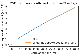
Retrained model MSD, diffusion coefficient¶

retrained_model_msd_job = get_msd_job(retrained_model_prod_md_job, "O")
retrained_model_D = (
    retrained_model_msd_job.results.get_diffusion_coefficient()
)  # diffusion coefficient, m^2/s
plot_msd(retrained_model_msd_job)

Reference MSD, diffusion coefficient¶

reference_msd_job = get_msd_job(reference_prod_md_job, "O")
reference_D = (
    reference_msd_job.results.get_diffusion_coefficient()
)  # diffusion coefficient, m^2/s
plot_msd(reference_msd_job)

Conclusion for diffusion coefficient: In this case, the retrained model gives 2.53e-9 m^2/s and the reference method 2.62e-9 m^2/s. That is very good agreement! Note: your results may be somewhat different.

Retrained model and reference RDF¶

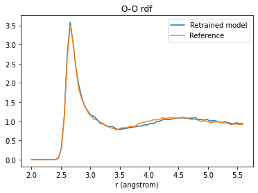
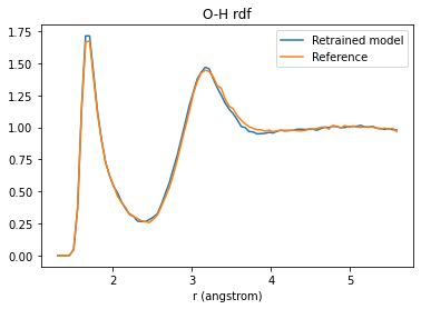
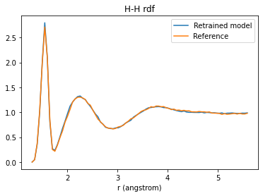
Let’s compare the calculated O-O, O-H, and H-H radial distribution functions (rdf):

def get_rdf(job, atom_indices, atom_indices_to, rmin, rmax, rstep):
    rdf = plams.AMSRDFJob(
        job,
        atom_indices=atom_indices,
        atom_indices_to=atom_indices_to,
        rmin=rmin,
        rmax=rmax,
        rstep=rstep,
    )
    rdf.run()

    return rdf.results.get_rdf()


final_frame = (
    retrained_model_prod_md_job.results.get_main_molecule()
)  # doesn't matter if retrained model or reference
O_ind = [i for i, at in enumerate(final_frame, 1) if at.symbol == "O"]
H_ind = [i for i, at in enumerate(final_frame, 1) if at.symbol == "H"]
rmax = final_frame.lattice[0][0] / 2
rstep = 0.05

O-O rdf¶

atom_indices, atom_indices_to = O_ind, O_ind
rmin = 2.0
pred_x, pred_y = get_rdf(
    retrained_model_prod_md_job, atom_indices, atom_indices_to, rmin, rmax, rstep
)
ref_x, ref_y = get_rdf(
    reference_prod_md_job, atom_indices, atom_indices_to, rmin, rmax, rstep
)
plt.plot(pred_x, pred_y, label="Retrained model")
plt.plot(ref_x, ref_y, label="Reference")
plt.xlabel("r (angstrom)")
plt.legend()
plt.title("O-O rdf");

O-H rdf¶

atom_indices, atom_indices_to = O_ind, H_ind
rmin = 1.3
pred_x, pred_y = get_rdf(
    retrained_model_prod_md_job, atom_indices, atom_indices_to, rmin, rmax, rstep
)
ref_x, ref_y = get_rdf(
    reference_prod_md_job, atom_indices, atom_indices_to, rmin, rmax, rstep
)
plt.plot(pred_x, pred_y, label="Retrained model")
plt.plot(ref_x, ref_y, label="Reference")
plt.xlabel("r (angstrom)")
plt.legend()
plt.title("O-H rdf");

H-H rdf¶

atom_indices, atom_indices_to = H_ind, H_ind
rmin = 1.3
pred_x, pred_y = get_rdf(
    retrained_model_prod_md_job, atom_indices, atom_indices_to, rmin, rmax, rstep
)
ref_x, ref_y = get_rdf(
    reference_prod_md_job, atom_indices, atom_indices_to, rmin, rmax, rstep
)
plt.plot(pred_x, pred_y, label="Retrained model")
plt.plot(ref_x, ref_y, label="Reference")
plt.xlabel("r (angstrom)")
plt.legend()
plt.title("H-H rdf");

Turn PLAMS logging back on¶

plams.config.log.stdout = 3  # default value

Density and NPT¶

Check the predicted vs. reference density¶

npt_md_s = plams.AMSNPTJob(
    nsteps=100000,
    timestep=0.5,
    thermostat="NHC",
    tau=100,
    temperature=300,
    barostat="MTK",
    barostat_tau=1000,
    equal="XYZ",
    pressure=1e5,
).settings

retrained_model_npt_job = plams.AMSJob(
    settings=npt_md_s + retrained_model_settings,
    name="retrained_model_npt",
    molecule=retrained_model_prod_md_job.results.get_main_molecule(),
)

retrained_model_npt_job.run();

[22.02|15:25:22] JOB retrained_model_npt STARTED
[22.02|15:25:22] JOB retrained_model_npt RUNNING
[22.02|16:06:01] JOB retrained_model_npt FINISHED
[22.02|16:06:01] JOB retrained_model_npt SUCCESSFUL

<scm.plams.interfaces.adfsuite.ams.AMSResults at 0x7fcc8c910670>

retrained_model_density = (
    plams.AMSNPTJob.load_external(retrained_model_npt_job.results.rkfpath())
    .results.get_equilibrated_molecule()
    .get_density()
)
print(
    f"Retrained model water density at 300 K: {retrained_model_density * 1e-3:.2f} g/cm^3"
)

Retrained model water density at 300 K: 0.95 g/cm^3

plams.config.jobmanager.hashing = None
reference_npt_job = plams.AMSJob(
    settings=npt_md_s + ref_s,
    name="reference_npt",
    molecule=reference_prod_md_job.results.get_main_molecule(),
)

reference_npt_job.run()

[22.02|18:53:54] JOB reference_npt STARTED
[22.02|18:53:54] Renaming job reference_npt to reference_npt.002
[22.02|18:53:54] JOB reference_npt.002 RUNNING
[22.02|18:58:13] JOB reference_npt.002 FINISHED
[22.02|18:58:13] JOB reference_npt.002 SUCCESSFUL

<scm.plams.interfaces.adfsuite.ams.AMSResults at 0x7fcc8d39d520>

reference_density = (
    plams.AMSNPTJob.load_external(reference_npt_job.results.rkfpath())
    .results.get_equilibrated_molecule()
    .get_density()
)
print(f"Reference model water density at 300 K: {reference_density * 1e-3:.2f} g/cm^3")

Reference model water density at 300 K: 1.01 g/cm^3

The above reference value for ReaxFF Water-2017.ff agrees exactly with the published reference value of 1.01 g/cm^3.

However, the retrained M3GNet model predicts a density of 0.95 g/cm^3. The agreement is reasonable but not excellent. This can be explained by the fact that almost all training data points were at 1.00 g/cm^3. Only a few points (from the “M3GNetShortMD” initial reference data generator) were taken at other densities.

Let’s continue the active learning while sampling more densities. There are two strategies:

Use an NPT simulation during the active learning
Scan the density during the active learning

Here, we choose the second approach in order to ensure that multiple different densities are sampled.

Initial structure for scanning density¶

Get the final frame from one of the previous MD simulations, and linearly scale the density to 800 kg/m^3 = 0.8 g/cm^3. This will stretch out the O-H bonds so follow up with a short UFF preoptimization.

new_structure = final_frame.copy()
new_structure.set_density(850)
new_structure = plams.preoptimize(new_structure, model="uff", maxiterations=20)

plams.plot_molecule(new_structure)

Second active learning job: scanning density¶

Here we set Steps.Type = “Linear” to run reference calculations every 5000 MD steps.

To get an accurate density it’s very important that the predicted energy is accurate. It is not enough to just get a good fit for the forces.

Here, we decrease the success criteria for both the energy and forces compared to default values.

nsteps = 80000
scan_density_md_s = plams.AMSMDScanDensityJob(
    molecule=new_structure,
    scan_density_upper=1.15,
    nsteps=nsteps,
    tau=100,
    thermostat="Berendsen",
    temperature=300,
).settings
# we must explicitly set the StopStep, since the AL divides the simulation into multiple segments
scan_density_md_s.input.ams.MolecularDynamics.Deformation.StopStep = nsteps

# job = SimpleActiveLearningJob.load_external(plams.config.default_jobmanager.workdir + "/sal.002")
scan_density_ml_s = ml_s.copy()
scan_density_ml_s.input.ams.MachineLearning.LoadModel = (
    job.results.get_params_results_directory()
)
scan_density_ml_s.input.ams.MachineLearning.Target.Forces.MAE = 0.02
scan_density_ml_s.input.ams.MachineLearning.MaxEpochs = 200

scan_density_al_s = plams.Settings()

scan_density_al_s.input.ams.ActiveLearning.Steps.Type = "Linear"
scan_density_al_s.input.ams.ActiveLearning.Steps.Linear.Start = 500
scan_density_al_s.input.ams.ActiveLearning.Steps.Linear.StepSize = 5000
scan_density_al_s.input.ams.ActiveLearning.InitialReferenceData.Load.FromPreviousModel = "Yes"

scan_density_al_s.input.ams.ActiveLearning.SuccessCriteria.Energy.Relative = 0.001
scan_density_al_s.input.ams.ActiveLearning.SuccessCriteria.Energy.Total = 0.002
# because we do not set Normalization, the above Energy criteria are energies per atom
# scan_density_al_s.input.ams.ActiveLearning.SuccessCriteria.Energy.Normalization =

scan_density_al_s.input.ams.ActiveLearning.SuccessCriteria.Forces.MaxDeviationForZeroForce = 0.30

scan_density_al_s.input.ams.ActiveLearning.AtEnd.RerunSimulation = "No"
scan_density_al_s.input.ams.ActiveLearning.MaxReferenceCalculationsPerAttempt = 2

scan_density_al_job = SimpleActiveLearningJob(
    name="scan_density_al",
    settings=ref_s + scan_density_md_s + scan_density_ml_s + scan_density_al_s,
    molecule=new_structure,
)
scan_density_al_job.run(watch=True);

[23.02|13:01:42] Simple Active Learning 2024.101,  Nodes: 1, Procs: 1
[23.02|13:01:44] Composition of main system: H96O48
[23.02|13:01:44] All REFERENCE calculations will be performed with the following ReaxFF engine:
[23.02|13:01:44]
Engine reaxff
... output trimmed ....



[23.02|14:07:16] Active learning finished!
[23.02|14:07:16] Goodbye!

Let’s recalculate the density again:

new_retrained_model_settings = scan_density_al_job.results.get_params_job().results.get_production_engine_settings()

new_retrained_model_npt_job = plams.AMSJob(
    settings=npt_md_s + new_retrained_model_settings,
    name="new_retrained_model_npt",
    molecule=retrained_model_prod_md_job.results.get_main_molecule(),
)

new_retrained_model_npt_job.run();

new_retrained_model_density = (
    plams.AMSNPTJob.load_external(new_retrained_model_npt_job.results.rkfpath())
    .results.get_equilibrated_molecule()
    .get_density()
)
print(
    f"New retrained model water density at 300 K: {new_retrained_model_density * 1e-3:.2f} g/cm^3"
)

New retrained model water density at 300 K: 1.02 g/cm^3

Conclusion for the density: Using active learning when scanning the densities makes sure that the predicitons are accurate for all densities. Consequently the equilibrium density is also in better agreement with the reference value of 1.01 g/cm^3.

Note that the density in general is quite difficult to fit accurately.

Python Script¶

#!/usr/bin/env python
# coding: utf-8

# When running active learning it's usually a good idea to start off "simple" and make the system/structures gradually more complicated.
#
# To train liquid water, we here
#
# * first train a potential at slightly above room temperature and 1.0 g/cm^3
#
# * continue with a second active learning loop where the density is explicitly scanned from a low to a high value
#
# ## Initial imports

import scm.plams as plams
from scm.simple_active_learning import SimpleActiveLearningJob
import matplotlib.pyplot as plt
from scm.external_engines.core import interface_is_installed

assert interface_is_installed("m3gnet"), "You must install the m3gnet backend before following this tutorial!"


plams.init()


# ## Create an initial water box

water = plams.from_smiles("O")
for at in water:
    at.properties = plams.Settings()
plams.plot_molecule(water)


box = plams.packmol(water, n_molecules=48, density=1.0)
plams.plot_molecule(box, rotation="-5x,5y,0z")


# Let's run a short MD simulation with M3GNet-UP-2022 to make the structure more realistic:

up_s = plams.Settings()
up_s.input.MLPotential.Model = "M3GNet-UP-2022"
up_s.runscript.nproc = 1  # always run AMS Driver in serial for MLPotential
up_md = plams.AMSNVTJob(
    molecule=box,
    settings=up_s,
    name="up_md",
    nsteps=1000,
    timestep=0.5,
    temperature=350,
)
up_md.run()
# New structure:

starting_structure = up_md.results.get_main_molecule()
plams.plot_molecule(starting_structure, rotation="-5x,5y,0z")


# ## Simple Active Learning setup
#
# ### Reference engine settings
#
# Here, we choose to train against ReaxFF Water-2017.ff, which gives a good water structure.

fast_ref_s = plams.Settings()
fast_ref_s.input.ReaxFF.ForceField = "Water2017.ff"
fast_ref_s.runscript.nproc = 1

slow_ref_s = plams.Settings()
slow_ref_s.input.QuantumESPRESSO.Pseudopotentials.Family = "SSSP-Efficiency"
slow_ref_s.input.QuantumESPRESSO.Pseudopotentials.Functional = "PBE"
slow_ref_s.input.QuantumESPRESSO.K_Points._h = "gamma"
slow_ref_s.input.QuantumESPRESSO.System = plams.Settings(
    input_dft="revpbe", ecutwfc=40, vdw_corr="Grimme-D3", dftd3_version=4
)


# Change to slow_ref_s to train to revPBE-D3(BJ) instead:

ref_s = fast_ref_s.copy()


# ### NVT molecular dynamics settings

nvt_md_s = plams.AMSNVTJob(
    nsteps=20000,
    timestep=0.5,
    temperature=(270, 350, 350),
    tau=100,
    thermostat="Berendsen",
).settings


# ### ParAMS machine learning settings

ml_s = plams.Settings()
ml_s.input.ams.MachineLearning.Backend = "M3GNet"
ml_s.input.ams.MachineLearning.CommitteeSize = 1
ml_s.input.ams.MachineLearning.M3GNet.Model = "UniversalPotential"
ml_s.input.ams.MachineLearning.MaxEpochs = 200


# ### Active learning settings
#
# Liquid water is a "simple" homogeneous system, so we can expect the ML method to perform quite well. We therefore decrease the success criteria thresholds a bit compared to the default vvalues, to ensure that we get accurate results.
#
# Since we will immediately continue with another active learning loop, we disable the "RerunSimulation" as we are not interested in the MD simulation per se.

al_s = plams.Settings()
al_s.input.ams.ActiveLearning.Steps.Type = "Geometric"
al_s.input.ams.ActiveLearning.Steps.Geometric.Start = 10
al_s.input.ams.ActiveLearning.Steps.Geometric.NumSteps = 8
al_s.input.ams.ActiveLearning.InitialReferenceData.Generate.M3GNetShortMD.Enabled = "Yes"
al_s.input.ams.ActiveLearning.SuccessCriteria.Energy.Relative = 0.003
al_s.input.ams.ActiveLearning.SuccessCriteria.Forces.MaxDeviationForZeroForce = 0.35
al_s.input.ams.ActiveLearning.AtEnd.RerunSimulation = "No"


# ### Complete job

settings = ref_s + nvt_md_s + ml_s + al_s
job = SimpleActiveLearningJob(settings=settings, molecule=starting_structure, name="sal")
print(job.get_input())


# ### Run the simple active learning job

job.run(watch=True)
# ## Validate trained model by RDF and MSD
#
# Note: You should skip this part if you trained to DFT since the reference MD calculation will take a very long time!

mol = job.results.get_main_molecule()
plams.plot_molecule(mol, rotation="-5x,5y,0z")


retrained_model_settings = job.results.get_params_job().results.get_production_engine_settings()
retrained_model_settings.runscript.nproc = 1


# ### Equilibration and production MD settings

eq_md_settings = plams.AMSNVTJob(
    nsteps=8000,
    timestep=0.5,
    thermostat="Berendsen",
    tau=100,
    temperature=300,
    samplingfreq=100,
).settings

prod_md_settings = plams.AMSNVTJob(
    nsteps=50000,
    timestep=0.5,
    thermostat="NHC",
    tau=200,
    temperature=300,
    samplingfreq=100,
).settings


# ### Retrained model equilibration

retrained_model_eq_md_job = plams.AMSJob(
    settings=eq_md_settings + retrained_model_settings,
    molecule=mol,
    name="retrained_model_eq_md_dens_1",
)
retrained_model_eq_md_job.run()
# ### Retrained model production simulation

# Let's then run a production simulation from the final structure of the above equilibration MD using both the retrained model and the reference engine:

retrained_model_prod_md_job = plams.AMSJob(
    settings=prod_md_settings + retrained_model_settings,
    name="retrained_model_prod_md_dens_1",
    molecule=retrained_model_eq_md_job.results.get_main_molecule(),
)
retrained_model_prod_md_job.run()
# ### Reference equilibration MD

reference_eq_md_job = plams.AMSJob(
    settings=eq_md_settings + ref_s,
    molecule=mol,
    name="reference_eq_md_dens_1",
)
reference_eq_md_job.run()
# ### Reference production MD

reference_prod_md_job = plams.AMSJob(
    settings=prod_md_settings + ref_s,
    name="reference_prod_md_dens_1",
    molecule=reference_eq_md_job.results.get_main_molecule(),
)
reference_prod_md_job.run()


# ### Mean squared displacement (MSD) helper functions

# For a detailed explanation of the MSD and RDF jobs, see the "Molecular dynamics with Python" tutorial


def get_msd_job(job: plams.AMSJob, symbol: str = "O"):
    atom_indices = [i for i, at in enumerate(job.results.get_main_molecule(), 1) if at.symbol == symbol]

    msd_job = plams.AMSMSDJob(
        job,
        name="msd-" + job.name,
        atom_indices=atom_indices,  # indices start with 1 for the first atom
        max_correlation_time_fs=4000,  # max correlation time must be set before running the job
        start_time_fit_fs=2000,  # start_time_fit can also be changed later in the postanalysis
    )
    msd_job.run()

    return msd_job


def plot_msd(job, start_time_fit_fs=None):
    """job: an AMSMSDJob"""
    time, msd = job.results.get_msd()
    fit_result, fit_x, fit_y = job.results.get_linear_fit(start_time_fit_fs=start_time_fit_fs)
    # the diffusion coefficient can also be calculated as fit_result.slope/6 (ang^2/fs)
    diffusion_coefficient = job.results.get_diffusion_coefficient(start_time_fit_fs=start_time_fit_fs)  # m^2/s
    plt.figure(figsize=(5, 3))
    plt.plot(time, msd, label="MSD")
    plt.plot(fit_x, fit_y, label="Linear fit slope={:.5f} ang^2/fs".format(fit_result.slope))
    plt.legend()
    plt.xlabel("Correlation time (fs)")
    plt.ylabel("Mean square displacement (ang^2)")
    plt.title("MSD: Diffusion coefficient = {:.2e} m^2/s".format(diffusion_coefficient))


plt.gcf().savefig("picture1.png")
plt.clf()


# ### Temporarily turn off PLAMS logging
#
# Technically, the MSD and RDF jobs are normal PLAMS jobs. However, they are very fast to run. We can turn off the PLAMS logging to keep the Jupyter notebook a bit more tidy:

plams.config.log.stdout = 0


# ### Retrained model MSD, diffusion coefficient

retrained_model_msd_job = get_msd_job(retrained_model_prod_md_job, "O")
retrained_model_D = retrained_model_msd_job.results.get_diffusion_coefficient()  # diffusion coefficient, m^2/s
plot_msd(retrained_model_msd_job)


# ### Reference MSD, diffusion coefficient

reference_msd_job = get_msd_job(reference_prod_md_job, "O")
reference_D = reference_msd_job.results.get_diffusion_coefficient()  # diffusion coefficient, m^2/s
plot_msd(reference_msd_job)


# **Conclusion for diffusion coefficient**: In this case, the retrained model gives 2.53e-9 m^2/s and the reference method 2.62e-9 m^2/s. That is very good agreement! Note: your results may be somewhat different.

# ### Retrained model and reference RDF
#
# Let's compare the calculated O-O, O-H, and H-H radial distribution functions (rdf):


def get_rdf(job, atom_indices, atom_indices_to, rmin, rmax, rstep):
    rdf = plams.AMSRDFJob(
        job,
        atom_indices=atom_indices,
        atom_indices_to=atom_indices_to,
        rmin=rmin,
        rmax=rmax,
        rstep=rstep,
    )
    rdf.run()

    return rdf.results.get_rdf()


final_frame = retrained_model_prod_md_job.results.get_main_molecule()  # doesn't matter if retrained model or reference
O_ind = [i for i, at in enumerate(final_frame, 1) if at.symbol == "O"]
H_ind = [i for i, at in enumerate(final_frame, 1) if at.symbol == "H"]
rmax = final_frame.lattice[0][0] / 2
rstep = 0.05


# ### O-O rdf

atom_indices, atom_indices_to = O_ind, O_ind
rmin = 2.0
pred_x, pred_y = get_rdf(retrained_model_prod_md_job, atom_indices, atom_indices_to, rmin, rmax, rstep)
ref_x, ref_y = get_rdf(reference_prod_md_job, atom_indices, atom_indices_to, rmin, rmax, rstep)
plt.plot(pred_x, pred_y, label="Retrained model")
plt.plot(ref_x, ref_y, label="Reference")
plt.xlabel("r (angstrom)")
plt.legend()
plt.title("O-O rdf")
plt.gcf().savefig("picture2.png")
plt.clf()


# ### O-H rdf

atom_indices, atom_indices_to = O_ind, H_ind
rmin = 1.3
pred_x, pred_y = get_rdf(retrained_model_prod_md_job, atom_indices, atom_indices_to, rmin, rmax, rstep)
ref_x, ref_y = get_rdf(reference_prod_md_job, atom_indices, atom_indices_to, rmin, rmax, rstep)
plt.plot(pred_x, pred_y, label="Retrained model")
plt.plot(ref_x, ref_y, label="Reference")
plt.xlabel("r (angstrom)")
plt.legend()
plt.title("O-H rdf")
plt.gcf().savefig("picture3.png")
plt.clf()


# ### H-H rdf

atom_indices, atom_indices_to = H_ind, H_ind
rmin = 1.3
pred_x, pred_y = get_rdf(retrained_model_prod_md_job, atom_indices, atom_indices_to, rmin, rmax, rstep)
ref_x, ref_y = get_rdf(reference_prod_md_job, atom_indices, atom_indices_to, rmin, rmax, rstep)
plt.plot(pred_x, pred_y, label="Retrained model")
plt.plot(ref_x, ref_y, label="Reference")
plt.xlabel("r (angstrom)")
plt.legend()
plt.title("H-H rdf")
plt.gcf().savefig("picture4.png")
plt.clf()


# ### Turn PLAMS logging back on

plams.config.log.stdout = 3  # default value


# ## Density and NPT
#
# ### Check the predicted vs. reference density

npt_md_s = plams.AMSNPTJob(
    nsteps=100000,
    timestep=0.5,
    thermostat="NHC",
    tau=100,
    temperature=300,
    barostat="MTK",
    barostat_tau=1000,
    equal="XYZ",
    pressure=1e5,
).settings


retrained_model_npt_job = plams.AMSJob(
    settings=npt_md_s + retrained_model_settings,
    name="retrained_model_npt",
    molecule=retrained_model_prod_md_job.results.get_main_molecule(),
)

retrained_model_npt_job.run()
retrained_model_density = (
    plams.AMSNPTJob.load_external(retrained_model_npt_job.results.rkfpath())
    .results.get_equilibrated_molecule()
    .get_density()
)
print(f"Retrained model water density at 300 K: {retrained_model_density * 1e-3:.2f} g/cm^3")


plams.config.jobmanager.hashing = None
reference_npt_job = plams.AMSJob(
    settings=npt_md_s + ref_s,
    name="reference_npt",
    molecule=reference_prod_md_job.results.get_main_molecule(),
)

reference_npt_job.run()


reference_density = (
    plams.AMSNPTJob.load_external(reference_npt_job.results.rkfpath()).results.get_equilibrated_molecule().get_density()
)
print(f"Reference model water density at 300 K: {reference_density * 1e-3:.2f} g/cm^3")


# The above reference value for ReaxFF Water-2017.ff agrees exactly with the published reference value of 1.01 g/cm^3.
#
# However, the retrained M3GNet model predicts a density of 0.95 g/cm^3. The agreement is reasonable but not excellent. This can be explained by the fact that almost all training data points were at 1.00 g/cm^3. Only a few points (from the "M3GNetShortMD" initial reference data generator) were taken at other densities.
#
# Let's continue the active learning while sampling more densities. There are two strategies:
#
# * Use an NPT simulation during the active learning
# * Scan the density during the active learning
#
# Here, we choose the second approach in order to ensure that multiple different densities are sampled.

# ### Initial structure for scanning density
#
# Get the final frame from one of the previous MD simulations, and linearly scale the density to 800 kg/m^3 = 0.8 g/cm^3. This will stretch out the O-H bonds so follow up with a short UFF preoptimization.

new_structure = final_frame.copy()
new_structure.set_density(850)
new_structure = plams.preoptimize(new_structure, model="uff", maxiterations=20)


plams.plot_molecule(new_structure)


# ### Second active learning job: scanning density
#
# Here we set Steps.Type = "Linear" to run reference calculations every 5000 MD steps.
#
# To get an accurate density it's very important that the predicted energy is accurate. It is not enough to just get a good fit for the forces.
#
# Here, we decrease the success criteria for both the energy and forces compared to default values.

nsteps = 80000
scan_density_md_s = plams.AMSMDScanDensityJob(
    molecule=new_structure,
    scan_density_upper=1.15,
    nsteps=nsteps,
    tau=100,
    thermostat="Berendsen",
    temperature=300,
).settings
# we must explicitly set the StopStep, since the AL divides the simulation into multiple segments
scan_density_md_s.input.ams.MolecularDynamics.Deformation.StopStep = nsteps


# job = SimpleActiveLearningJob.load_external(plams.config.default_jobmanager.workdir + "/sal.002")
scan_density_ml_s = ml_s.copy()
scan_density_ml_s.input.ams.MachineLearning.LoadModel = job.results.get_params_results_directory()
scan_density_ml_s.input.ams.MachineLearning.Target.Forces.MAE = 0.02
scan_density_ml_s.input.ams.MachineLearning.MaxEpochs = 200


scan_density_al_s = plams.Settings()

scan_density_al_s.input.ams.ActiveLearning.Steps.Type = "Linear"
scan_density_al_s.input.ams.ActiveLearning.Steps.Linear.Start = 500
scan_density_al_s.input.ams.ActiveLearning.Steps.Linear.StepSize = 5000
scan_density_al_s.input.ams.ActiveLearning.InitialReferenceData.Load.FromPreviousModel = "Yes"

scan_density_al_s.input.ams.ActiveLearning.SuccessCriteria.Energy.Relative = 0.001
scan_density_al_s.input.ams.ActiveLearning.SuccessCriteria.Energy.Total = 0.002
# because we do not set Normalization, the above Energy criteria are energies per atom
# scan_density_al_s.input.ams.ActiveLearning.SuccessCriteria.Energy.Normalization =

scan_density_al_s.input.ams.ActiveLearning.SuccessCriteria.Forces.MaxDeviationForZeroForce = 0.30

scan_density_al_s.input.ams.ActiveLearning.AtEnd.RerunSimulation = "No"
scan_density_al_s.input.ams.ActiveLearning.MaxReferenceCalculationsPerAttempt = 2


scan_density_al_job = SimpleActiveLearningJob(
    name="scan_density_al",
    settings=ref_s + scan_density_md_s + scan_density_ml_s + scan_density_al_s,
    molecule=new_structure,
)
scan_density_al_job.run(watch=True)
# Let's recalculate the density again:

new_retrained_model_settings = scan_density_al_job.results.get_params_job().results.get_production_engine_settings()

new_retrained_model_npt_job = plams.AMSJob(
    settings=npt_md_s + new_retrained_model_settings,
    name="new_retrained_model_npt",
    molecule=retrained_model_prod_md_job.results.get_main_molecule(),
)

new_retrained_model_npt_job.run()
new_retrained_model_density = (
    plams.AMSNPTJob.load_external(new_retrained_model_npt_job.results.rkfpath())
    .results.get_equilibrated_molecule()
    .get_density()
)
print(f"New retrained model water density at 300 K: {new_retrained_model_density * 1e-3:.2f} g/cm^3")


# **Conclusion for the density**: Using active learning when scanning the densities makes sure that the predicitons are accurate for all densities. Consequently the equilibrium density is also in better agreement with the reference value of 1.01 g/cm^3.
#
# Note that the density in general is quite difficult to fit accurately.