
Thermal conductivity from NEMD
Calculate thermal conductivity from non-equilibrium molecular dynamics. For details, see the corresponding GUI tutorial.
Downloads: Notebook | Script ?
Additional files required by this example:
BBO_COF1.xyz
Requires: AMS2027 or later
Related examples
Related tutorials
Related documentation
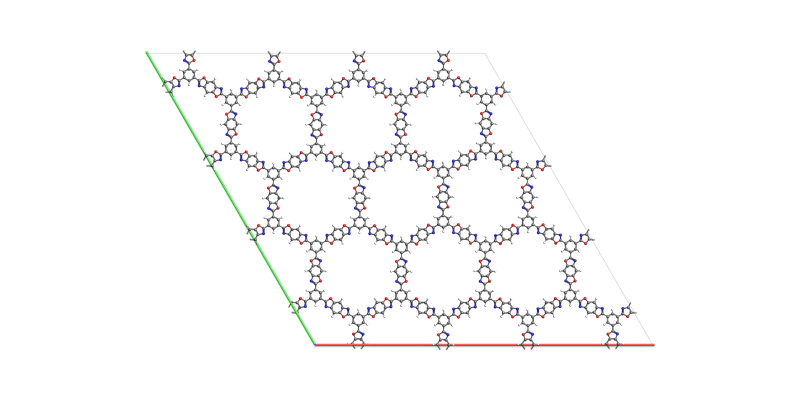
Load and visualize the initial system
from scm.base import ChemicalSystem
from scm.plams import view, ViewConfig

# dependency: {} BBO_COF1.xyz

BBO_COF1 = ChemicalSystem.from_file('BBO_COF1.xyz')
BBO_COF1.guess_bonds()
vcfg = ViewConfig(show_regions=True, width=800, height=600, padding=-20, show_lattice_vectors=True)
img = view(BBO_COF1, config=vcfg)
img
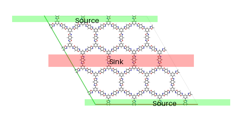
Clarify what are the sink and source regions
The view of a chemical system is a PIL image and can thus be annotated for scientific communication.
Here, we add Source and Sink labels to the image. In the next section, we assign those atoms to regions that can be used in the simulation.
from PIL import ImageDraw, Image

tmp = Image.new('RGBA', img.size)
draw = ImageDraw.Draw(tmp)


draw.rectangle([(img.width*0.2, img.height*.45), (img.width*0.8, img.height*.55)],
fill=(255, 0, 0, 80))

draw.rectangle([(img.width*0.05, img.height*.13), (img.width*0.65, img.height*0.18)],
fill=(0, 255, 0, 80))
draw.rectangle([(img.width*0.35, img.height*.82), (img.width*0.95, img.height*0.87)],
fill=(0, 255, 0, 80))

draw.text((img.width*0.451, img.height*0.47), "Sink", (0, 0, 0), font_size=24)

draw.text((img.width*0.31, img.height*0.13), "Source", (0, 0, 0), font_size=24)
draw.text((img.width*0.63, img.height*0.815), "Source", (0, 0, 0), font_size=24)

out = Image.alpha_composite(img, tmp)
out
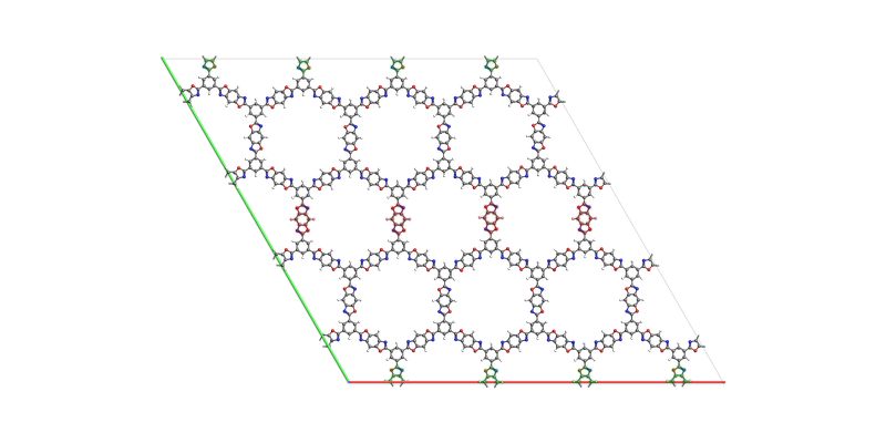
Assign atoms to source and sink regions
The XYZ file used in the GUI tutorial does not contain regions, so assign atoms to the source and sink regions from their positions along the y direction. These selections reproduce the regions in the supplied BBO_COF1.in reference structure. Region colors are assigned automatically and may differ from the GUI tutorial.
for atom in BBO_COF1:
    if atom.coords[1] <= 3.39 or atom.coords[1] >= 69.00:
        BBO_COF1.add_atom_to_region(atom, 'source')
    if 32.9 <= atom.coords[1] <= 39.7:
        BBO_COF1.add_atom_to_region(atom, 'sink')

view(BBO_COF1, config=vcfg)
Set up simulation settings
Set thermostats for sink and source
source_stat = {
    "Region": "source",
    "Tau": "10.0",  # fs
    "Temperature": "90.0",  # K
    "Type": "NHC",
}

# Only the region and temperature of the sink thermostat are different.
sink_stat = source_stat.copy()
sink_stat["Region"] = "sink"
sink_stat["Temperature"] = "70.0"
Setup MD with UFF
from scm.inputs import AMS, ForceField

s = AMS(Task="MolecularDynamics")
s.Engine = ForceField()
s.MolecularDynamics.NSteps = 200000
s.MolecularDynamics.TimeStep = 1.0
s.MolecularDynamics.InitialVelocities.Temperature = 80.0
s.MolecularDynamics.Thermostat = [source_stat, sink_stat]
s.MolecularDynamics.Trajectory.SamplingFreq = 1000
s.MolecularDynamics.Trajectory.EngineResultsFreq = 0
Run the job
from scm.plams import AMSJob

job = AMSJob(settings=s, molecule=BBO_COF1)
results = job.run();

#job = AMSJob.load('plams_workdir/plamsjob') sometimes it is convenient to load and analyse a previously obtained simulation
#results = job.results
[12.10|10:04:58] JOB plamsjob STARTED
[12.10|10:04:58] JOB plamsjob RUNNING
[12.10|10:20:00] JOB plamsjob FINISHED
[12.10|10:20:01] JOB plamsjob SUCCESSFUL
Analyze the results and extract thermal conductivity
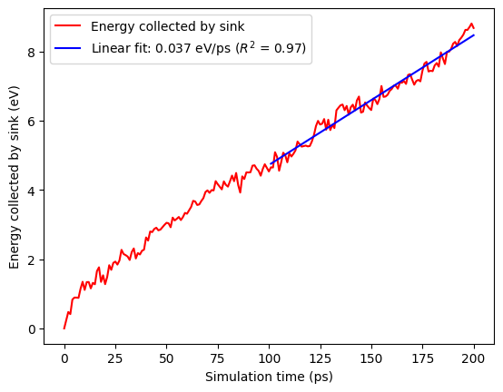
Obtain the energy collected by the sink thermostat as a function of time. Because the sink is the second thermostat in the input, its energy is stored as NHCTstat2Energy. After equilibration, this energy should increase approximately linearly with time.
from scm.base import Units
import numpy as np
from matplotlib import pyplot as plt

time = results.get_history_property("Time", history_section="MDHistory")
time = np.array(time)*Units.conversion_factor('fs', 'ps')

nhctstatenergy = results.get_history_property("NHCTstat2Energy", history_section="MDHistory")
nhctstatenergy = np.array(nhctstatenergy)*Units.conversion_factor('hartree', 'eV')

equilibrium = time > 100 # Here it is assumed that the system is in equilibrium after 100ps, this needs proper investigation for each calculation.
a, b = np.polyfit(time[equilibrium], nhctstatenergy[equilibrium], deg=1)
r_squared = np.corrcoef(time[equilibrium], nhctstatenergy[equilibrium])[0, 1] ** 2

fig, ax = plt.subplots()
ax.set_xlabel('Simulation time (ps)')
ax.set_ylabel('Energy collected by sink (eV)')
ax.plot(time, nhctstatenergy, 'red', label='Energy collected by sink')
ax.plot(time[equilibrium], a * time[equilibrium] + b, 'blue', label=f'Linear fit: {a:.3f} eV/ps ($R^2$ = {r_squared:.2f})')
ax.legend()
ax;
Now we can obtain the thermal conductivity \(k\)
from IPython.display import display, Markdown

dEdT = a * Units.conversion_factor('eV', 'J') / Units.conversion_factor('ps', 's')
display(Markdown(rf'$\frac{{dE}}{{dt}}$ = {dEdT:.3e} W'))
print(f'dE/dt = {dEdT:.3e} W')
\(\frac{dE}{dt}\) = 6.007e-09 W
dE/dt = 6.007e-09 W
va, vb, vc = BBO_COF1.lattice.vectors
L = np.linalg.norm(vb[1])/2*Units.conversion_factor('Angstrom', 'm')
display(Markdown(rf'$L$={L:.3e} m'))
print(f'L = {L:.3e} m')
\(L\)=3.615e-09 m
L = 3.615e-09 m
S = np.linalg.norm(np.cross(np.asarray(va).T, vc))*Units.conversion_factor('Angstrom', 'm')**2
display(Markdown(rf'$S$={S:.3e} m${{}}^2$'))
print(f'S = {S:.3e} m^2')
\(S\)=2.820e-18 m\({}^2\)
S = 2.820e-18 m^2
thermostats = job.settings.input.MolecularDynamics.Thermostat
dT = abs(float(thermostats[0].Temperature[0]) - float(thermostats[1].Temperature[0]))
display(Markdown(rf'$\Delta T$={dT:.3f} K'))
print(f'Delta T = {dT:.3f} K')
\(\Delta T\)=20.000 K
Delta T = 20.000 K
k = dEdT*L/(2*S*dT)
display(Markdown(rf'$k$={k:.3f} W m${{}}^{{-1}}$ K${{}}^{{-1}}$'))
print(f'k = {k:.3f} W m^-1 K^-1')
\(k\)=0.193 W m\({}^{-1}\) K\({}^{-1}\)
k = 0.193 W m^-1 K^-1
The GUI tutorial obtains approximately 0.23 W m\(^{-1}\) K\(^{-1}\). The exact value varies slightly because the thermostatted MD simulation is non-deterministic and the trajectory is relatively short.
See also
Python Script
#!/usr/bin/env python
# coding: utf-8

# ## Load and visualize the initial system

from scm.base import ChemicalSystem
from scm.plams import view, ViewConfig

# dependency: {} BBO_COF1.xyz

BBO_COF1 = ChemicalSystem.from_file('BBO_COF1.xyz')
BBO_COF1.guess_bonds()


vcfg = ViewConfig(show_regions=True, width=800, height=600, padding=-20, show_lattice_vectors=True)
img = view(BBO_COF1, config=vcfg)
img


# ## Clarify what are the sink and source regions

# The view of a chemical system is a [PIL](https://pillow.readthedocs.io/en/stable/) image and can thus be annotated for scientific communication.
#
# Here, we add Source and Sink labels to the image. In the next section, we assign those atoms to regions that can be used in the simulation.

from PIL import ImageDraw, Image

tmp = Image.new('RGBA', img.size)
draw = ImageDraw.Draw(tmp)


draw.rectangle([(img.width*0.2, img.height*.45), (img.width*0.8, img.height*.55)],
fill=(255, 0, 0, 80))

draw.rectangle([(img.width*0.05, img.height*.13), (img.width*0.65, img.height*0.18)],
fill=(0, 255, 0, 80))
draw.rectangle([(img.width*0.35, img.height*.82), (img.width*0.95, img.height*0.87)],
fill=(0, 255, 0, 80))

draw.text((img.width*0.451, img.height*0.47), "Sink", (0, 0, 0), font_size=24)

draw.text((img.width*0.31, img.height*0.13), "Source", (0, 0, 0), font_size=24)
draw.text((img.width*0.63, img.height*0.815), "Source", (0, 0, 0), font_size=24)

out = Image.alpha_composite(img, tmp)
out


# ## Assign atoms to source and sink regions

# The XYZ file used in the GUI tutorial does not contain regions, so assign atoms to the `source` and `sink` regions from their positions along the y direction. These selections reproduce the regions in the supplied `BBO_COF1.in` reference structure. Region colors are assigned automatically and may differ from the GUI tutorial.

for atom in BBO_COF1:
    if atom.coords[1] <= 3.39 or atom.coords[1] >= 69.00:
        BBO_COF1.add_atom_to_region(atom, 'source')
    if 32.9 <= atom.coords[1] <= 39.7:
        BBO_COF1.add_atom_to_region(atom, 'sink')

view(BBO_COF1, config=vcfg, picture_path="picture1.png")


# ## Set up simulation settings

# Set thermostats for sink and source

source_stat = {
    "Region": "source",
    "Tau": "10.0",  # fs
    "Temperature": "90.0",  # K
    "Type": "NHC",
}

# Only the region and temperature of the sink thermostat are different.
sink_stat = source_stat.copy()
sink_stat["Region"] = "sink"
sink_stat["Temperature"] = "70.0"


# Setup MD with UFF

from scm.inputs import AMS, ForceField

s = AMS(Task="MolecularDynamics")
s.Engine = ForceField()
s.MolecularDynamics.NSteps = 200000
s.MolecularDynamics.TimeStep = 1.0
s.MolecularDynamics.InitialVelocities.Temperature = 80.0
s.MolecularDynamics.Thermostat = [source_stat, sink_stat]
s.MolecularDynamics.Trajectory.SamplingFreq = 1000
s.MolecularDynamics.Trajectory.EngineResultsFreq = 0


# ## Run the job

from scm.plams import AMSJob

job = AMSJob(settings=s, molecule=BBO_COF1)
results = job.run();

#job = AMSJob.load('plams_workdir/plamsjob') sometimes it is convenient to load and analyse a previously obtained simulation
#results = job.results


# ## Analyze the results and extract thermal conductivity

# Obtain the energy collected by the sink thermostat as a function of time. Because the sink is the second thermostat in the input, its energy is stored as `NHCTstat2Energy`. After equilibration, this energy should increase approximately linearly with time.

from scm.base import Units
import numpy as np
from matplotlib import pyplot as plt

time = results.get_history_property("Time", history_section="MDHistory")
time = np.array(time)*Units.conversion_factor('fs', 'ps')

nhctstatenergy = results.get_history_property("NHCTstat2Energy", history_section="MDHistory")
nhctstatenergy = np.array(nhctstatenergy)*Units.conversion_factor('hartree', 'eV')

equilibrium = time > 100 # Here it is assumed that the system is in equilibrium after 100ps, this needs proper investigation for each calculation.
a, b = np.polyfit(time[equilibrium], nhctstatenergy[equilibrium], deg=1)
r_squared = np.corrcoef(time[equilibrium], nhctstatenergy[equilibrium])[0, 1] ** 2

fig, ax = plt.subplots()
ax.set_xlabel('Simulation time (ps)')
ax.set_ylabel('Energy collected by sink (eV)')
ax.plot(time, nhctstatenergy, 'red', label='Energy collected by sink')
ax.plot(time[equilibrium], a * time[equilibrium] + b, 'blue', label=f'Linear fit: {a:.3f} eV/ps ($R^2$ = {r_squared:.2f})')
ax.legend()
ax;
ax.figure.savefig("picture2.png")


# Now we can obtain the thermal conductivity $k$
#
# $$
# k = \frac{dE}{dT} \frac{L}{ 2S\Delta T}
# $$


dEdT = a * Units.conversion_factor('eV', 'J') / Units.conversion_factor('ps', 's')
print(f'dE/dt = {dEdT:.3e} W')


va, vb, vc = BBO_COF1.lattice.vectors
L = np.linalg.norm(vb[1])/2*Units.conversion_factor('Angstrom', 'm')
print(f'L = {L:.3e} m')


S = np.linalg.norm(np.cross(np.asarray(va).T, vc))*Units.conversion_factor('Angstrom', 'm')**2
print(f'S = {S:.3e} m^2')


thermostats = job.settings.input.MolecularDynamics.Thermostat
dT = abs(float(thermostats[0].Temperature[0]) - float(thermostats[1].Temperature[0]))
print(f'Delta T = {dT:.3f} K')


k = dEdT*L/(2*S*dT)
print(f'k = {k:.3f} W m^-1 K^-1')


# The GUI tutorial obtains approximately 0.23 W m$^{-1}$ K$^{-1}$. The exact value varies slightly because the thermostatted MD simulation is non-deterministic and the trajectory is relatively short.