PEDA-NOCV - decomposing the orbital relaxation term
This tutorial will teach you how to perform a Periodic Energy Decomposition Analysis (PEDA) combined with the Natural Orbitals for Chemical Valency (NOCV) method for periodic systems with BAND. It will also show how to visualize NOCV orbitals and NOCV deformation densities.
Setting up the System and the Calculation
Preparations for the PEDA-NOCV calculation
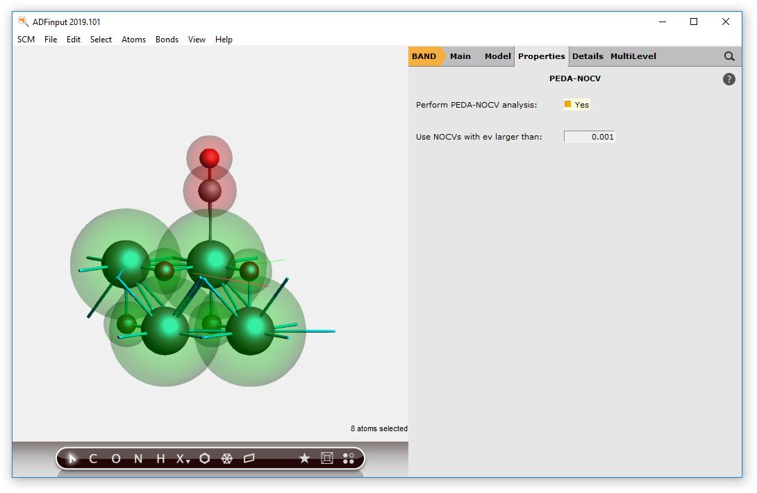
Now the PEDA-NOCV has to be switched on. Go to the PEDA-NOCV menu,
You may want to define a NOCV eigenvalue threshold (default: 0.001) which handles the amount of output.
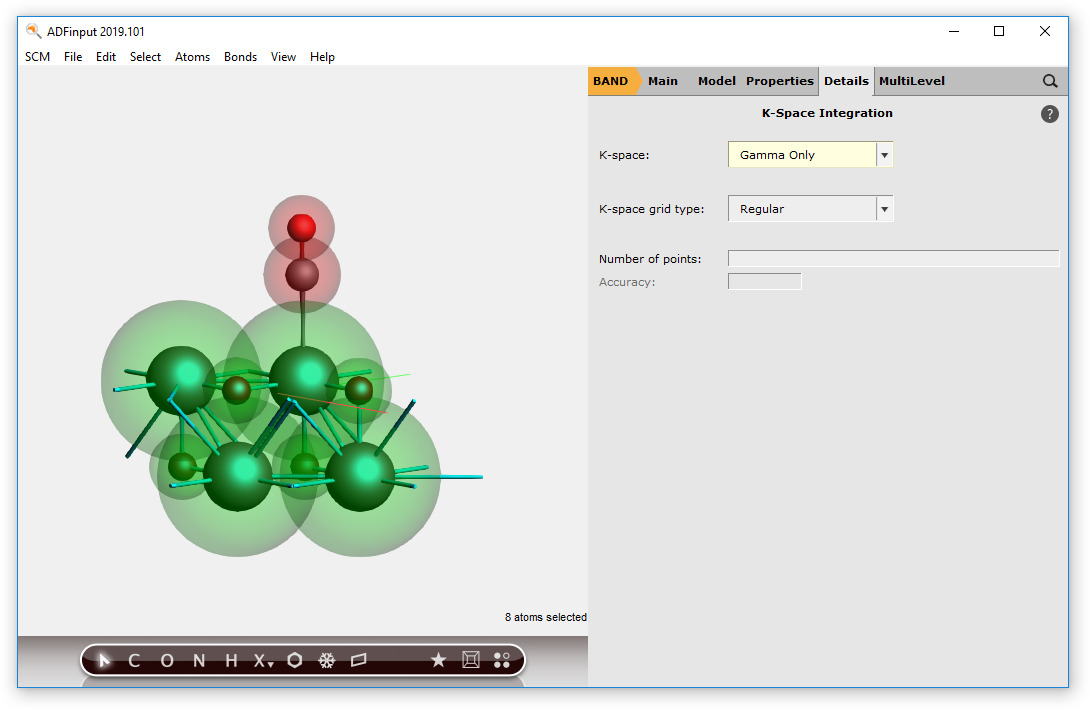
Then you have to keep in mind that the PEDA-NOCV is implemented for \(\Gamma\)-only case. So, go to the ‘Integration K-Space’ menu,
Save and run the calculation
Now you can save and run the calculation.
Step 2: Checking the results
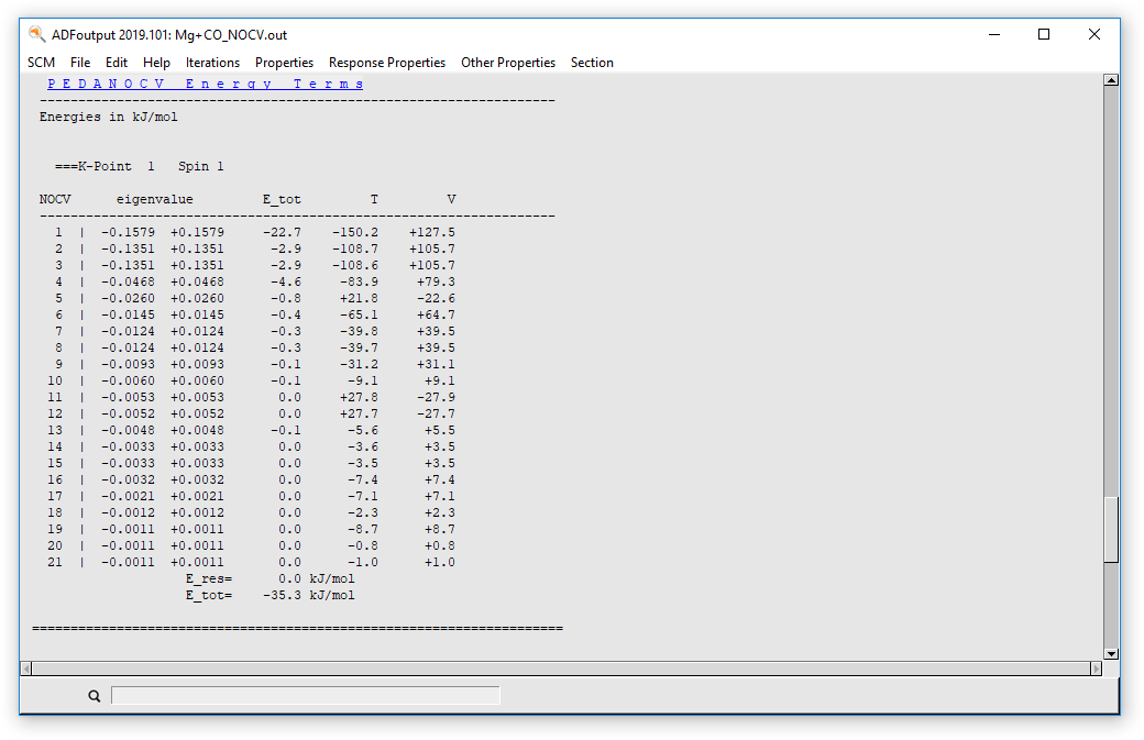
After the calculations of the fragments and the PEDA finished you can look for the PEDA results. Therefore, open the “Output” using the SCM dropdown menu.
You can jump to the ‘PEDA-NOCV Energy Terms’ via the corresponding button in the ‘Properties’ drop-down menu.
Reference results:
Step 3: Plotting NOCV orbitals and deformation densities
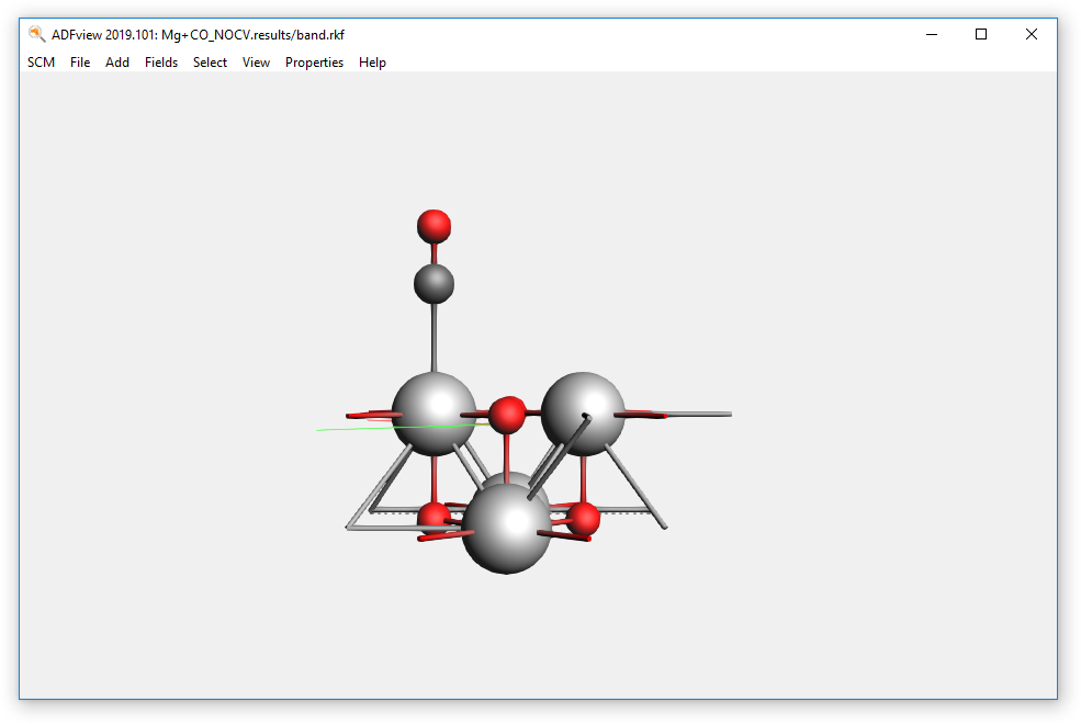
You can visualize the charge NOCV deformation densities which describe the charge flow between the fragments. Therefore, open the “View” using the SCM drop-down menu.
Depending on your preferences (w.r.t. showing atoms of neighboring cells) you will end up with the following representation of AMSview.
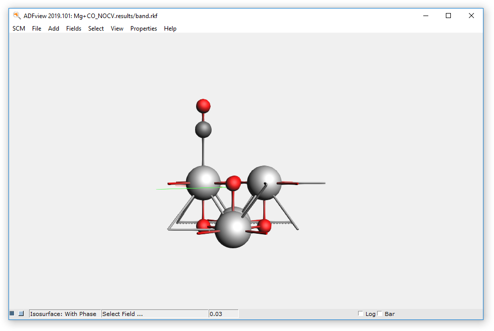
You can now add an isosurface with phase via the drop-down menu ‘Add’, or via ‘Ctrl+B’.
Step 3a: Plotting NOCV deformation densities
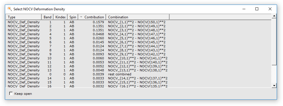
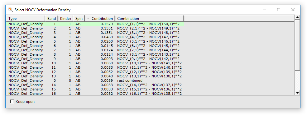
To get an overview of the NOCV deformation densities click on ‘Select Field …’ and then on ‘NOCV Def Densities…’. The following window should appear.
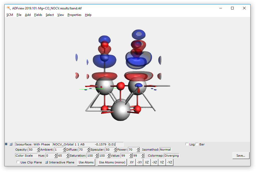
For example you can now visualize the first NOCV deformation density. (Be aware of the small isovalue of 0.000025 in the following picture!)
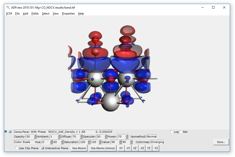
(For further tweaking you can click on “Isosurface: With Phase” and select “Show Details”)
This deformation density visualizes the charge flow from red to blue lobes. Here, the charge transfer from the CO to the MgO surface is shown.
According to the information in the ‘Select NOCV Deformation Density’ window the first NOCV deformation density is a combination of the NOCV orbitals 1 (the small number denotes the donor/occupied NOCV) and 150 (the large number denotes the acceptor/unoccupied NOCV).
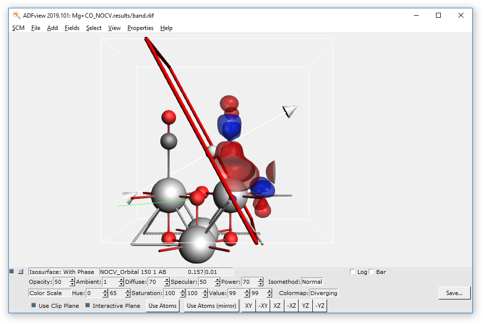
Step 3b: Plotting NOCV orbitals
These NOCV orbitals can visualized by changing the field to ‘NOCV Orbitals’. The following window should appear.
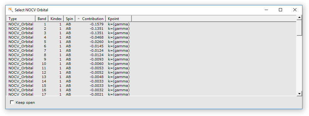
By selecting the 1st and 150th NOCV orbital these are calculated and can then be visualized one at a time.
NOCV orbital 1 does show predominantly a lone-pair localized at the CO fragment.
NOCV orbital 150 does show predominantly a lobe connecting the CO fragment and a Mg atom of the surface.
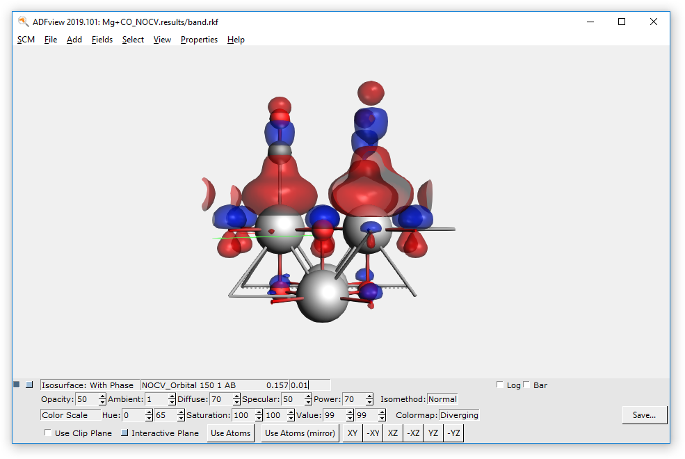
Remark: The calculated fields for the NOCV properties does represent not only the central unit cell but partially the neighboring cells. So, it can be tough to only show what is needed and not confuse additional lobes of the neighboring cells with something in the unit cell! You can hide parts of the field using the Clip Plane in BANDGUI.
To optimize the resulting plot one can visualize (temporarily) and modify the position of the Clip Plane by checking Interactive Plane.