Work functions at interfaces¶

This tutorial will show how to use BAND to calculate the work function Φ of the

Al(100)/vacuum interface
Al(100)/LiF(100) interface

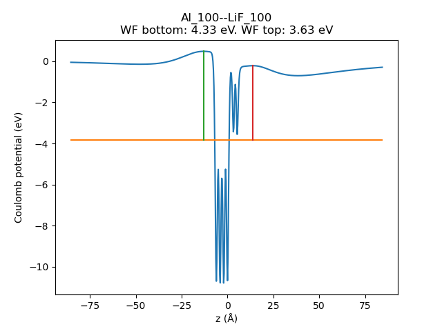
../_images/preview19.png — Fig. 45 Plane-averaged electrostatic (Coulomb) potential vs z coordinate. The orange horizontal line is the Fermi energy. The red and green vertical lines indicate how the work function is calculated on either side of the slab. The work function (WF) for the Al(100)/vacuum interface (green) is 4.33 eV. The WF for the Al(100)/LiF(100) interface (red) is 3.63 eV.¶

In the above figure the work function Φ is calculated as

Φ = local maximum in Coulomb potential - Fermi energy

The adsorption of LiF(100) will decrease the work function, as compared to vacuum. The results will be compared to plane-wave-DFT results by Prada S., et al. 1 and Kondo and Matsushista 2

	Al(100) Φ [eV]	Al(100)/LiF(100) ΔΦ [eV]	functional	code
Prada et al.	4.37	-0.7	PW91	VASP
Kondo and Matsushista	4.28	-0.59	PBE	Quantum ESPRESSO
This tutorial	4.33	-0.70	PW91	BAND

Note

The above works differ not only in code and functional, but also basis set, k-point sampling, number of layers in the Al or LiF slabs, whether the system is relaxed or not, …

Build the initial system¶

Start AMSinput

Switch to BAND:

→

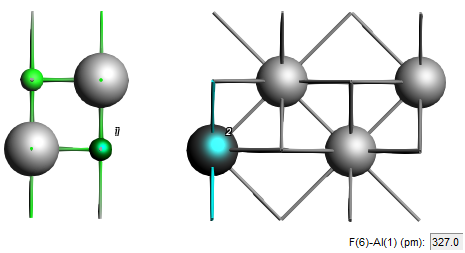
When setting up a solid-solid interface, the lattice constants must match. Both Al and LiF are cubic, so if their lattice constants match, also the (100) surface lattice constants will match. At least one of the materials needs to be a bit strained. Here, we will strain the LiF slab to match the Al slab. We will place the LiF slab at a distance of 3.27 Å from the Al slab.

Note

For other interfaces, you may need to apply surface rotations and use surface supercells if the lattice constants of the two materials are very different, in order to not apply too much strain to one of the materials.

Download the LiF-on-Al.xyz file

Select File → Import Coordinates and select the downloaded file

See also

If you are not yet familiar with the editing tools in AMSinput, take a look at our Introduction to Building structures.

First, build the Al(100) slab:

Edit → Crystal → Cubic → fcc
Choose Al from the drop-down, note the lattice constant a = 4.05 Å.
Edit → Crystal → Generate Slab
Click the Convert to Conventional Cell button
Leave Number of layers at 2
Click Generate Slab to generate a 4-layer Al(001) (equivalent to Al(100)) slab

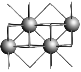
Similarly, open a new AMSinput window and create the LiF(100) slab:

SCM → New Input
Edit → Crystal → Cubic → NaCl
Choose LiF from the drop-down
Set the lattice constant to 4.05 Å (the same value as for the Al slab)
Click OK
Edit → Crystal → Generate Slab
Click the Convert to conventional cell button
Set the number of layers to 1
Click Generate slab. This gives a 2-layer LiF(100) slab.

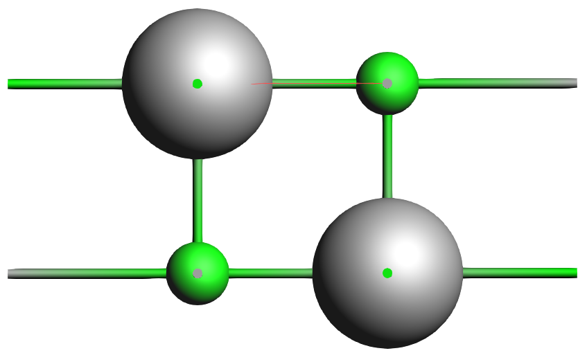
We now want to position this LiF slab on top of the Al slab such that the F atom is 3.27 Å directly above the top Al atom

Select all atoms in the LiF slab
Hold the right mouse button and drag them up a bit so that the bottom atoms are above the ab plane (this way they will not overlap the Al slab when you combine the two systems)
Edit → Copy
Switch to the Al(100) AMSinput window
Edit → Paste
Unselect all atoms
Edit → Tune Geometry
Select the bottom F atom. Hold shift and click on the other three LiF atoms (selecting them)
Click the ⬭ next to Atoms to move

Click the top Al atom (selecting only this atom)
Click the ⬭  next to Above atoms
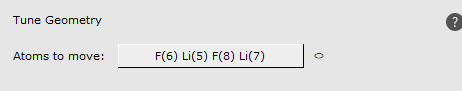
Distance to plane: 3.27 Å to first atom (the first atom is the first selected F atom)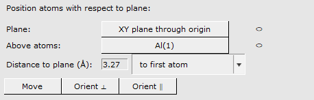
Click the Move button
Click Close

This has created the desired interface geometry.

Set up the DFT calculation¶

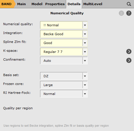
Then, set the BAND settings:

XC functional: GGA → PW91
Basis set: DZP
Details → Numerical Quality
Integration: Becke Good
Spline Zlm fit: Good

Click the

next to K-space

Number of points: 7 7

Details → SCF

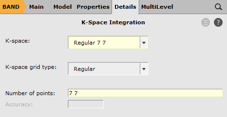
Electronic temperature: 0.002 hartree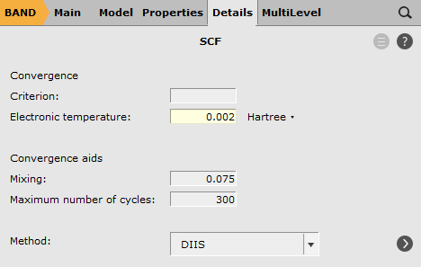

This sets up a 7x7 k-space grid. The integration, spline zlm fit, and electronic temperature options help with the SCF convergence.

Save and run the job.

File → Save As with a new name

Run the job

Get work function with Python script¶

Download WorkFunctionVacuumAndInterface.py
Modify the results_dir variable to give the correct path to the .results folder from the previous calculation. It should contain two files: ams.rkf and band.rkf.
Open a terminal and run the script as $AMSBIN/amspython WorkFunctionVacuumAndInterface.py

This produces a plot like the below:

Get work function with the graphical user interface¶

Select the job in AMSjobs and select SCM → View
Fields → Grid → Full Unit Cell
Fields → Grid → Details…
In the popup window, set  Grid extends beyond molecule in z direction to: 100 Å
Click Use

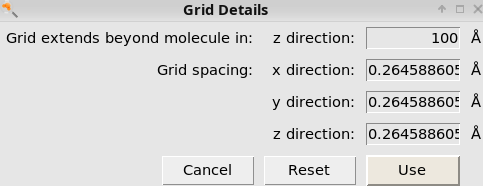
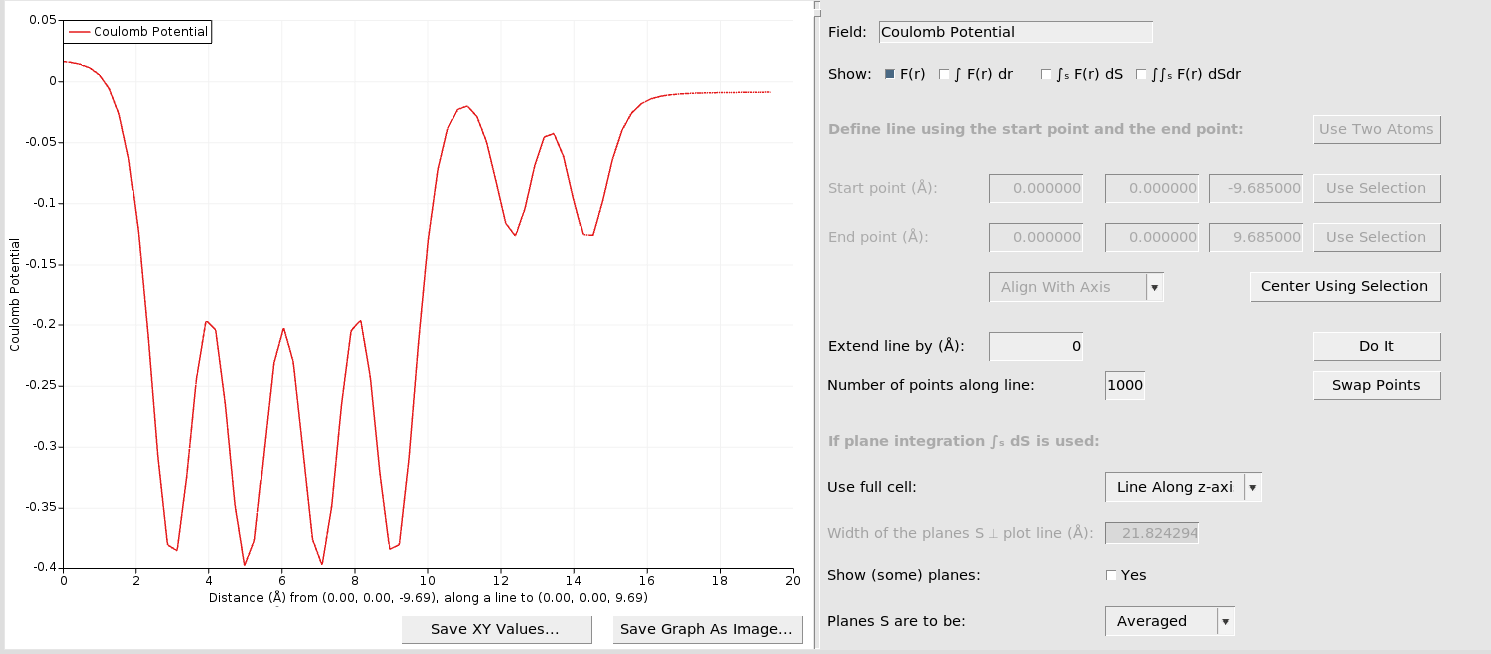
Then, switch to the line graph generator:

Add → Graph Along Line
Extend line by (Å): 0
Number of points along line: 1000
In the Use full cell: dropdown menu, select Line Along z-axis
In the Planes S are to be dropdown menu, select Averaged
In the Field drop-down menu at the top, select Potential → Coulomb Potential

This produces the following plot:

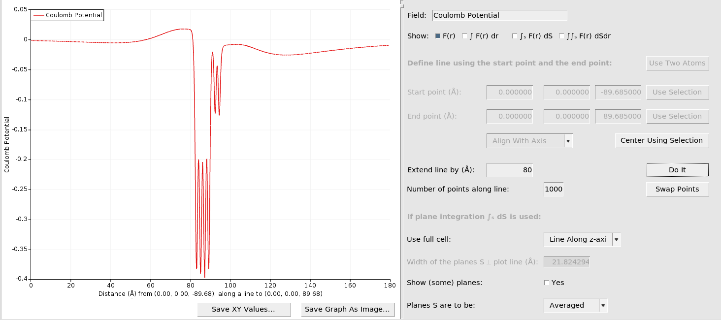
To extend the plotted potential further out into the vacuum:

Extend line by (Å): 80

Click the Do it button next to Extend line by (Å)

Note that the extension which here is set to 80, which needs to be smaller than the “Grid extends beyond molecule” previously set to 100.

This should produce a figure like the following:

If you hover over the first and second local maxima at the left hand-side, you can read off the y coordinates as

left-hand side (bottom side of slab, Al/vacuum): 0.0176 hartree
right-hand side (top side of slab, Al/LiF): -0.0081 hartree

These plane-averaged potentials should be compared to the Fermi energy to get the work function.

SCM → Output

In AMSoutput, do Properties → Band gap information

This gives:

Band gap information

 No band gap

 Fermi Energy:    -0.1413 a.u.
 Fermi Energy:    -3.8443 eV

Consequently, we get

bottom side Φ = 0.02555 - (-0.1413) = 0.16685 hartree = 4.33 eV
top side Φ = -0.0081 - (-0.1413) = 0.1332 hartree = 3.62 eV

1

Prada, U Martinez, G. Pacchioni. Work function changes induced by deposition of ultrathin dielectric films on metals: A theoretical analysis. Phys. Rev. B. 78, 235423. DOI: 10.1103/PhysRevB.78.235423

2

Kondo, T. Matsushista. Vacuum-Level Shift at Al/LiF/Alq3 Interfaces: A First-Principles Study. ACS Omega 2019, 4, 8, 13426–13434. https://doi.org/10.1021/acsomega.9b01667