Sensitivity Analysis¶

GloMPO implements a sensitivity analysis method to aid in reducing the dimensionality of high-dimensional optimization problems. The Hilbert-Schmidt Independence Criterion (HSIC) is the chosen method due to its robustness and accuracy.

The analysis module comes with three main components:

Class	Description
`HSIC`	Performs the sensitivity calculation
`HSICResult`	Result of a sensitivity calculation
`BaseKernel`	Base class of the kernels needed by `HSIC`

HSIC¶

class HSIC(x, y, labels=None, x_bounds='auto')[source]¶

Implementation of the Hilbert-Schmidt Independence Criterion for global sensitivity analysis. Estimates the HSIC via the unbiased estimator of Song et al (2012).

Parameters

x: \(n \times d\) matrix of \(d\)-dimensional vectors in the input space. These are samples of the variables you would like to know the sensitivity for.
y: \(n\) length vector of outputs corresponding to the input samples in x. These are the responses of some function against which the sensitivity is measured.
labels: Optional list of factor names.
x_bounds: \(d \times 2\) matrix of min-max pairs for every factor in x to scale the values between 0 and 1. Defaults to 'auto' which takes the limits as the min and max values of the sample data. To use no scaling set this to None.

Notes

y is automatically scaled by taking the logarithm of the values and then scaling by the minimum and maximum to a range between zero and one. This makes selecting kernel parameters easier, and deals with order-of-magnitude problems which often arise during reparameterization.

References

Song, L., Smola, A., Gretton, A., Bedo, J., & Borgwardt, K. (2012). Feature Selection via Dependence Maximization. Journal of Machine Learning Research, 13, 1393–1434. https://doi.org/10.5555/2188385.2343691

Gretton, A., Bousquet, O., Smola, A., & Schölkopf, B. (2005). Measuring Statistical Dependence with Hilbert-Schmidt Norms. In Lecture Notes in Computer Science (including subseries Lecture Notes in Artificial Intelligence and Lecture Notes in Bioinformatics): Vol. 3734 LNAI (Issue 140, pp. 63–77). Springer, Berlin, Heidelberg. https://doi.org/10.1007/11564089_7

Gretton, A., Borgwardt, K. M., Rasch, M. J., Smola, A., Schölkopf, B., Smola GRETTON, A., & Smola, A. (2012). A kernel two-sample test. Journal of Machine Learning Research, 13(25), 723–773. http://jmlr.org/papers/v13/gretton12a.html

Spagnol, A., Riche, R. Le, & Veiga, S. Da. (2019). Global Sensitivity Analysis for Optimization with Variable Selection. SIAM/ASA Journal on Uncertainty Quantification, 7(2), 417–443. https://doi.org/10.1137/18M1167978

Da Veiga, S. (2015). Global sensitivity analysis with dependence measures. Journal of Statistical Computation and Simulation, 85(7), 1283–1305. https://doi.org/10.1080/00949655.2014.945932

compute(inputs_kernel=None, outputs_kernel=None, n_bootstraps=1, n_sample=- 1, replace=False)[source]¶

Calculates the HSIC for each input factor. The larger the HSIC value for a parameter, the more sensitive y is to changes in the corresponding parameter in x.

Parameters

inputs_kernel: Instance of BaseKernel which will be applied to x. Defaults to GaussianKernel.
outputs_kernel: Instance of BaseKernel which will be applied to y. Defaults to ConjunctiveGaussianKernel.
n_bootstraps: Number of repeats of the calculation with different sub-samples from the data set. A small spread from a large number of bootstraps provides confidence on the estimation of the sensitivity.
n_sample: Number of vectors in x to use in the calculation. Defaults to -1 which uses all available points.
replace: If True, samples from x will be done with replacement and vice verse. This only has an effect if n_sample is less than n otherwise replace is True by necessity.

Returns

HSICResult: Object containing the results of the HSIC calculation and the calculation settings.

compute_with_reweight(residuals, targets, error_weights, error_sigma, inputs_kernel=None, outputs_kernel=None, n_bootstraps=1, n_sample=- 1, replace=False, max_cache_size=None)[source]¶

Computes the sensitivity of the HSIC to the weights applied to the construction of an error function. This calculation is only applicable in very particular conditions:

\(X \in \mathbb{R}^{n \times d}\) represents the inputs to a function which produces \(m\) outputs for each \(d\) length input vector input of \(X\) resampled \(n\) times.
These outputs are the \(n \times m\) predictions matrix (\(P\)).
The predictions matrix can be condensed to the \(n\) length vector y by an ‘error’ function:

\[\mathbf{y} = \sum^d_i w_i \left(\frac{P_i - r_i}{\sigma_i}\right)^2\]
\(\mathbf{r}\), \(\mathbf{w}\) and \(\mathbf{\sigma}\) are \(m\) length vectors of reference, error_weights, and error_sigma values respectively.
This function returns \(\frac{dg}{d\mathbf{w}}\) which is a measure of how much changes in \(\mathbf{w}\) (the ‘weights’ in the error function) will affect \(g\) which is a measure of how close HSIC values are to our target HSIC sensitivities.
\(g\) is defined such that \(g \geq 0\). \(g = 0\) implies the sensitivities are perfect.

Parameters

residuals: \(n \times m\) matrix of error values between predictions and references.
targets: \(d\) length boolean vector. If an element is True, one would like the corresponding parameter to show sensitivity. Can also send a vector of real values such that sum of elements is 1. This allows for custom sensitivities to be targeted for each parameter.
error_weights: \(m\) length vector of error function ‘weights’ for which the sensitivity will be measured.
error_sigma: \(m\) length vector of error function ‘standard error’ values.
inputs_kernel: See compute(). But only one value is allowed in this function.
outputs_kernel: See compute().
n_bootstraps: Number of repeats of the calculation with different sub-samples from the data set. A small spread from a large number of bootstraps provides confidence on the estimation of the sensitivity.
n_sample: Number of vectors in x to use in the calculation. Defaults to -1 which uses all available points.
replace: If True, samples from x will be done with replacement and vice verse. This only has an effect if n_sample is less than n otherwise replace is True by necessity.
max_cache_size: Maximum amount of disk space (in bytes) the program may use to store matrices and speed-up the calculation. Defaults to the maximum size of the temporary directory on the system.

Returns

HSICResultWithReweight: Object containing the results of the HSIC calculation and the calculation settings.

Warning

Efforts have been made to reduce the memory footprint of the calculation, but it can become very large, very quickly.

This calculation is also significantly slower than the normal sensitivity calculation.

HSIC Results¶

class HSICResult(*args, **kwargs)[source]¶

Result object of a single HSIC calculation produced by HSIC.compute(). Can only be created by HSIC.compute() or load().

__str__(top_n=5, width=50)[source]¶: Returns a summary of the result and its settings.

property hsic¶

\(d\) vector of raw HSIC calculation results. If n_bootstraps is larger than one, this represents the mean over the bootstraps.

See Also

hsic_std sensitivities

property hsic_std¶

\(d\) vector of the standard deviation of raw HSIC calculation results across all the bootstraps.

See Also

hsic sensitivities_std

property inputs_kernel¶: Name of the kernel applied to the input-space data.

property inputs_kernel_parameters¶: Parameters for the input kernel.

classmethod load(path)[source]¶

Load a calculation result from file.

Parameters

path: Path to saved result file

See Also

save()

property n_bootstraps¶: Number of times the HSIC calculation was performed with different sub-samples of the data.

property n_factors¶: Number of factors analyzed.

property n_samples¶: Number of items in the sub-samples of the data used in each bootstrap.

property order_factors¶

Returns factor indices in descending order of their influence on the outputs. The positions in the array are the rankings, the contents of the array are the factor indices. This is the inverse of ranking().

Returns

numpy.ndarray: \(d\) vector of order factors.

See Also

ranking

property outputs_kernel¶: Name of the kernel applied to the output-space data.

property outputs_kernel_parameters¶: Parameters for the output kernel.

plot_grouped_sensitivities(path='trend.png', squash_threshold=0.0, _seed_ax=None)[source]¶

Create a pie chart of the sensitivities result per factor group. Assumes labels for the parameters take the format: group:factor_name.

Parameters

path: Optional file location in which to save the image. If not provided the image is not saved and only returned.
squash_threshold: If a group’s sensitivity falls below this value it will be added to the ‘Other’ wedge of the plot.

Returns

matplotlib.figure.Figure: Figure instance allowing the user to further tweak and change the plot as desired.

plot_sensitivities(path='hsicresult.png', plot_top_n=None)[source]¶

Create a detailed graphic of the sensitivities results.

Parameters

path: Optional file location in which to save the image. If not provided the image is not saved and only returned.
plot_top_n: The number of factors to include in the plot. Only the plot_top_n most influential factors are included.

Returns

matplotlib.figure.Figure: Figure instance allowing the user to further tweak and change the plot as desired.

plot_sensitivity_trends(path='trend.png', _seed_ax=None)[source]¶

Create a summary graphic of the sensitivities results. This is a more abstract version of plot_sensitivities() that always includes all parameters. It is useful to inspect the sensitivity imbalance between parameters as well as the spread between repeats.

Parameters

path: Optional file location in which to save the image. If not provided the image is not saved and only returned.

Returns

matplotlib.figure.Figure: Figure instance allowing the user to further tweak and change the plot as desired.

property ranking¶

Returns the ranking of each factor being analyzed. The positions in the array are the factor indices, the contents of the array are rankings such that 1 is the most influential factor and \(g+1\) is the least influential. This is the inverse of order_factors().

Returns

numpy.ndarray: \(d\) vector of rankings.

See Also

order_factors

property sampling_with_replacement¶: Whether sampling was done with or without replacement from the available data. False, if all available data was used and automatically True if more samples were used than the number available in the data set.

save(path='hsiccalc.npz')[source]¶

Saves the result to file. Uses the numpy '.npz' format to save the result attributes (see numpy.savez).

Parameters

path: Path to file in which the result will be saved.

property sensitivities¶

\(d\) vector of normalised HSIC calculation results. These are the main sensitivity results a user should be concerned with. If n_bootstraps is larger than one. This represents the mean over the bootstraps.

Sensitivities are defined such that:

\[\sum S_d = 1\]

\[0 \leq S_d \leq 1\]

See Also

hsic sensitivities_std

property sensitivities_std¶

\(d\) vector of the standard deviation of normalised HSIC calculation results across all the bootstraps.

See Also

hsic_std sensitivities

class HSICResultWithReweight(*args, **kwargs)[source]¶

Bases: scm.glompo.analysis.hsic.HSICResult

property dg¶: \(n_{bootstraps} \times m\) matrix of gradients of \(g\) with respect to the \(m\) weights in the data set.

property g¶: Metric of the sensitivity imbalance (\(g\)). \(g \geq 0\) such that \(g = 0\) means all sensitivities are on target. If n_bootstraps is larger than one. This represents the mean over the bootstraps.

property g_std¶: Standard deviation of \(g\) across all the bootstraps. Returns None if a reweight calculation was not run.

property n_residuals¶: Returns the number of residuals contributing to the loss function.

plot_reweight(path='reweightresult.png', group_by=None, labels=None)[source]¶

Create a graphic of the reweight results.

Parameters

path: Optional file location in which to save the image. If not provided the image is not saved and only returned.
group_by: Sequence of integer indices grouping individual loss function contributions by training set item. For example, all the forces in a single data set ‘Forces’ item.
labels: Sequence of data set item names.

Returns

matplotlib.figure.Figure: Figure instance allowing the user to further tweak and change the plot as desired.

save_reweight_summary(path='reweightresult.csv', group_by=None, labels=None)[source]¶

Save a summary of the reweight calculation to a text file.

Parameters

group_by: Sequence of integer indices grouping individual loss function contributions by training set item. For example, all the forces in a single data set ‘Forces’ item.
labels: Sequence of data set item names.

suggest_weights(group_by=None, return_stats=False)[source]¶

Suggest new weights based on the reweight calculation results. If n_bootstraps is larger than one, uses the mean dg value over the bootstraps.

Parameters

group_by: Sequence of integer indices grouping individual loss function contributions by training set item. For example, all the forces in a single data set ‘Forces’ item.

property targets¶: \(d\) length vector of target sensitivity values for each parameter. Returns None if a reweight calculation was not run.

property weights¶: Original \(m\) length vector of weights used in the loss function. Returns None if a reweight calculation was not run.

Kernels¶

Kernels are the key inputs for the sensitivity calculation.

One kernel is applied to the parameters for which the sensitivity is being tested.
One kernel is applied to the function values the sensitivity is being tested against.

Note

Sensitivities are calculated for one parameter at a time, hence the kernels below are not multi-dimensional since their inputs are always scaler values.

class BaseKernel[source]¶

__call__(*args)[source]¶

Returns the kernel value or the derivative depending on the number of arguments.

See Also

compute() derivative()

abstract compute(data)[source]¶

Returns the kernel value given a set of data.

Parameters

data: Vector of data onto which the kernel will be applied. The kernel will be applied to the outer combination of data elements.

derivative(y, dy)[source]¶

Returns the first derivative of the kernel with respect to the weights used in the loss function.

Parameters

y: Vector of data points. The outer combination of all points will be calculated.
dy: First derivative of y with respect to the weights used in the loss function.

class ConjunctiveGaussianKernel(gamma=0.1)[source]¶

Bases: scm.glompo.analysis.kernels.BaseKernel

Sigmoid type kernel, similar to the ThresholdKernel, but continuous. Places the bulk of the distribution on the data points with the lowest values.

\[k(x, y) = \exp\left[ - \frac{x^2 + y^2}{2\gamma^2} \right]\]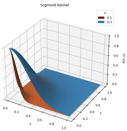

Parameters

gamma: Higher values extend the distribution over more points (\(0 < \gamma < 1\)).

class GaussianKernel(sigma=0.3)[source]¶

Bases: scm.glompo.analysis.kernels.BaseKernel

Traditional Gaussian kernel used to measure the similarity between inputs.

\[k(x, y) = \exp\left[ - \frac{(x - y)^2}{2\sigma^2} \right]\]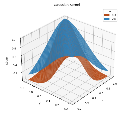

Parameters

sigma: Normal distribution bandwidth parameter (\(0 < \sigma < 1\))

class LinearKernel[source]¶

Bases: scm.glompo.analysis.kernels.PolynomialKernel

Special instance of PolynomialKernel of degree 1 and shift 0.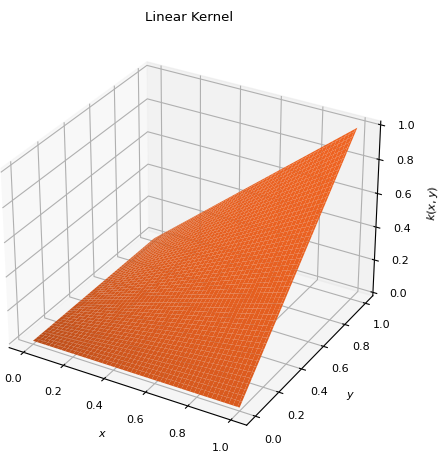

\[k(x, y) = x y\]

class PolynomialKernel(order=1, shift=0)[source]¶

Bases: scm.glompo.analysis.kernels.BaseKernel

Polynomial kernel which places the distribution bulk on the highest data values.

\[k(x, y) = (x y + c)^d\]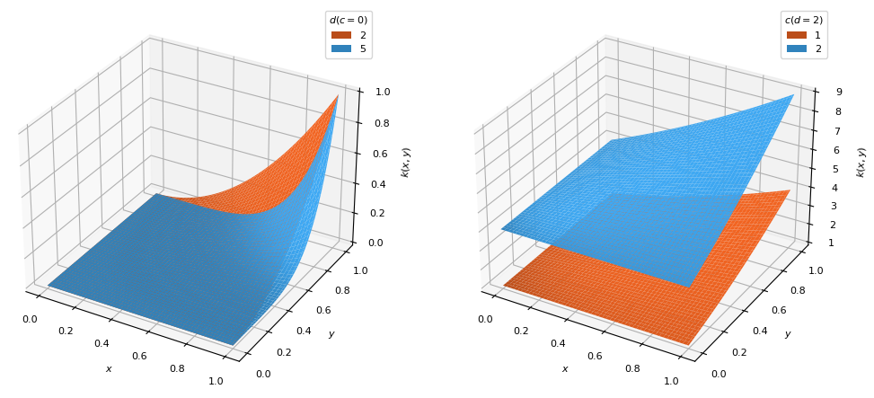

Parameters

order: Degree (\(d\)) of the polynomial function (\(d \geq 1\))
shift: Vertical shift (\(c\)) of the distribution to temper the effects of order

class ThresholdKernel(alpha)[source]¶

Bases: scm.glompo.analysis.kernels.BaseKernel

Simple linear kernel which first toggles the data to zero or one. Places the distribution over the smallest function values.

\[\begin{split}g(x) = \begin{cases} 1 &\text{ if } x < q_\alpha \\ 0 &\text{ if } x \geq q_\alpha \\ \end{cases}\end{split}\]

\[k(x, y) = g(x) g(y)\]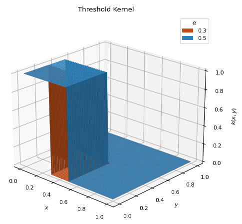

Parameter

alpha: Sets all values below the alpha quantile in data to 1 and all those above to 0 (\(0 < \alpha < 1\)).

References

Spagnol, A., Riche, R. Le, & Veiga, S. Da. (2019). Global Sensitivity Analysis for Optimization with Variable Selection. SIAM/ASA Journal on Uncertainty Quantification, 7(2), 417–443. https://doi.org/10.1137/18M1167978