Basic molecular dynamics analysis

Note: This example requires AMS2023 or later.

This example illustrates how to calculate the basic

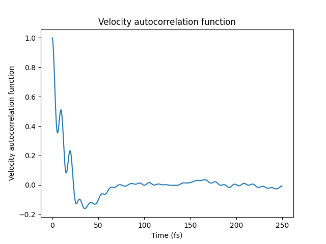
• velocity autocorrelation function (VACF)

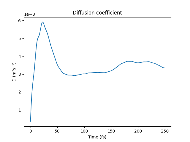
• diffusion coefficient from the integral of the VACF

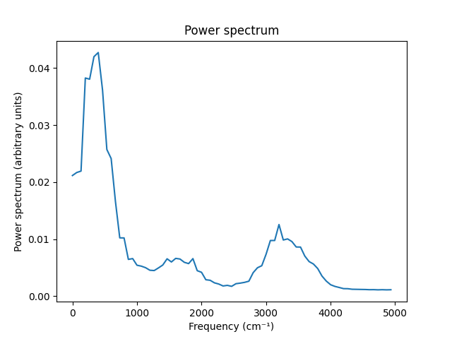
• power spectrum (Fourier transform of the VACF)

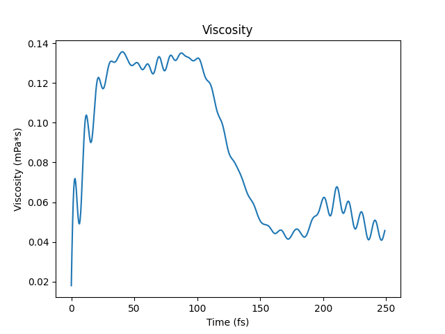
• viscosity from the Green-Kubo relation (integral of the off-diagonal pressure tensor autocorrelation function)

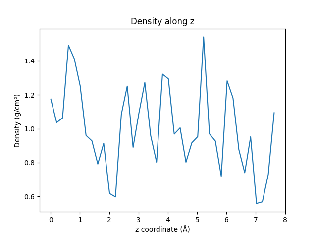
• density along the z axis

For details about the functions, see the AMSResults API.

Technical

The example only shows how to technically calculate the numbers. For real simulations, run longer MD simulations and carefully converge any calculated quantities.

The viscosity requires especially long MD simulations.

Note

More advanced analysis is possible by setting up an AMSAnalysisJob job.

See also: Molecular Dynamics with Python

Example usage: (Download BasicMDPostanalysis.py)

#!/usr/bin/env plams
import os

import matplotlib.pyplot as plt
import numpy as np
from scm.plams import *


def run_md():
    mol = packmol(from_smiles("O"), n_molecules=16, density=1.0)
    s = Settings()
    s.input.ams.Task = "MolecularDynamics"
    s.input.ReaxFF.ForceField = "Water2017.ff"
    s.input.ams.MolecularDynamics.CalcPressure = "Yes"
    s.input.ams.MolecularDynamics.InitialVelocities.Temperature = 300
    s.input.ams.MolecularDynamics.Trajectory.SamplingFreq = 1
    s.input.ams.MolecularDynamics.TimeStep = 0.5
    s.input.ams.MolecularDynamics.NSteps = 2000
    s.runscript.nproc = 1
    os.environ["OMP_NUM_THREADS"] = "1"
    job = AMSJob(settings=s, molecule=mol, name="md")
    job.run()
    return job


def plot_results(results):
    plt.clf()
    times, vacf = results.get_velocity_acf(start_fs=0, max_dt_fs=250, normalize=False)
    normalized_vacf = vacf / vacf[0]
    plt.plot(times, normalized_vacf)
    plt.xlabel("Time (fs)")
    plt.ylabel("Velocity autocorrelation function")
    plt.title("Velocity autocorrelation function")
    plt.savefig("plams_vacf.png")
    A = np.stack((times, normalized_vacf), axis=1)
    np.savetxt("plams_vacf.txt", A, header="Time(fs) VACF")

    plt.clf()
    t_D, D = results.get_diffusion_coefficient_from_velocity_acf(times, vacf)
    plt.plot(t_D, D)
    plt.xlabel("Time (fs)")
    plt.ylabel("D (m²s⁻¹)")
    plt.title("Diffusion coefficient")
    plt.savefig("plams_vacf_D.png")
    A = np.stack((t_D, D), axis=1)
    np.savetxt("plams_vacf_D.txt", A, header="time(fs) D(m^2*s^-1)")

    plt.clf()
    freq, intensities = results.get_power_spectrum(times, vacf, number_of_points=1000)
    plt.plot(freq, intensities)
    plt.xlabel("Frequency (cm⁻¹)")
    plt.ylabel("Power spectrum (arbitrary units)")
    plt.title("Power spectrum")
    plt.savefig("plams_power_spectrum.png")
    A = np.stack((freq, intensities), axis=1)
    np.savetxt("plams_power_spectrum.txt", A, header="Frequency(cm^-1) PowerSpectrum")

    plt.clf()
    t, viscosity = results.get_green_kubo_viscosity(start_fs=0, max_dt_fs=250)  # do not do this for NPT simulations
    plt.plot(t, viscosity)
    plt.xlabel("Time (fs)")
    plt.ylabel("Viscosity (mPa*s)")
    plt.title("Viscosity")
    plt.savefig("plams_green_kubo_viscosity.png")
    A = np.stack((t, viscosity), axis=1)
    np.savetxt("plams_green_kubo_viscosity.txt", A, header="Time(fs) Viscosity(mPa*s)")

    plt.clf()
    z, density = results.get_density_along_axis(axis="z", density_type="mass", bin_width=0.2, atom_indices=None)
    plt.plot(z, density)
    plt.xlabel("z coordinate (Å)")
    plt.ylabel("Density (g/cm³)")
    plt.title("Density along z")
    plt.savefig("plams_density_along_z.png")
    A = np.stack((z, density), axis=1)
    np.savetxt("plams_density_along_z.txt", A, header="z(angstrom) density(g/cm^3)")


def main():
    job = run_md()
    # alternatively:
    # job = AMSJob.load_external('/path/to/ams.rkf')
    plot_results(job.results)


if __name__ == "__main__":
    main()