Phase Transitions in the ZGB model.¶

Note

To follow this tutorial, either:

Download PhaseTransitions.py (run as $AMSBIN/amspython PhaseTransitions.py).
Download PhaseTransitions.ipynb (see also: how to install Jupyterlab)

This example is inspired in the seminal paper: Kinetic Phase Transitions in an Irreversible Surface-Reaction Model by Robert M. Ziff, Erdagon Gulari, and Yoav Barshad in 1986 Phys. Rev. Lett. 56, (1986) 2553. The authors proposed a simple model for catalytic reactions of carbon monoxide oxidation to carbon dioxide on a surface. This model is now known as the Ziff-Gulari-Barshad (ZGB) model after their names. While the model leaves out many important steps of the real system, it exhibits interesting steady-state off-equilibrium behavior and two types of phase transitions, which actually occur in real systems. Please refer to the original paper for more details. In this example, we will analyze the effect of changing the composition of the gas phase, namely partial pressures for $O_2$ and $CO$, in the $CO_2$ Turnover frequency (TOF) in the ZGB model.

The first step is to import all packages we need:

import multiprocessing
import numpy
import scm.plams
import scm.pyzacros as pz

First must define the system. So, we have to specify species, lattice, cluster expansion, and mechanisms. As we said above, we will use the ZGB model, which consists on:

1. Three gas species: $CO$, $O_2$, and $CO_2$. Notice that the gas_energy by default is zero unless otherwise stated. That’s the case for $CO$ and $O2$, which are used as energy references.

CO_gas = pz.Species("CO")
O2_gas = pz.Species("O2")
CO2_gas = pz.Species("CO2", gas_energy=-2.337)

2. Three surface species: $*$, $CO^*$, $O^*$. The species $*$ represents the empty adsorption site. All of them have denticity equal to 1.

s0 = pz.Species("*", 1)
CO_ads = pz.Species("CO*", 1)
O_ads = pz.Species("O*", 1)

3. A rectangular lattice with a single site type.

lattice = pz.Lattice( lattice_type=pz.Lattice.RECTANGULAR, lattice_constant=1.0, repeat_cell=[50,50] )

4. Two clusters in the cluster-expansion Hamiltonian: $CO^*$-bs and $O^*$-bs. They are attached to a single binding site. No lateral interactions are considered.

CO_point = pz.Cluster(species=[CO_ads], energy=-1.3)
O_point = pz.Cluster(species=[O_ads], energy=-2.3)

cluster_expansion = [CO_point, O_point]

5. Three irreversible events: adsorption of $CO$, dissociative adsorption of $O_2$, and $CO$ oxidation.

# CO_adsorption:
CO_adsorption = pz.ElementaryReaction(initial=[s0,CO_gas],
                                      final=[CO_ads],
                                      reversible=False,
                                      pre_expon=10.0,
                                      activation_energy=0.0)

# O2_adsorption:
O2_adsorption = pz.ElementaryReaction(initial=[s0,s0,O2_gas],
                                      final=[O_ads,O_ads],
                                      neighboring=[(0, 1)],
                                      reversible=False,
                                      pre_expon=2.5,
                                      activation_energy=0.0)

# CO_oxidation:
CO_oxidation = pz.ElementaryReaction(initial=[CO_ads, O_ads],
                                     final=[s0, s0, CO2_gas],
                                     neighboring=[(0, 1)],
                                     reversible=False,
                                     pre_expon=1.0e+20,
                                     activation_energy=0.0)

mechanism = [CO_adsorption, O2_adsorption, CO_oxidation]

Now, we initialize the pyZacros environment.

scm.pyzacros.init()

PLAMS working folder: /home/user/pyzacros/examples/ZiffGulariBarshad/plams_workdir

This calculation is relatively fast. On a typical laptop, it should take around 1 min to complete. However, to illustrate how to run several in parallel Zacros calculations, we’ll use the plams.JobRunner class, which easily allows us to run as many parallel instances as we request. In this case, we choose to use the maximum number of simultaneous processes (maxjobs) equal to the number of processors in the machine. Additionally, by setting nproc = 1 we establish that only one processor will be used for each zacros instance.

maxjobs = multiprocessing.cpu_count()
scm.plams.config.default_jobrunner = scm.plams.JobRunner(parallel=True, maxjobs=maxjobs)
scm.plams.config.job.runscript.nproc = 1
print('Running up to {} jobs in parallel simultaneously'.format(maxjobs))

Running up to 8 jobs in parallel simultaneously

Now we have to set up the calculation using a Settings object. Firstly, we set a reactants gas phase composition of 45% $CO$ and 55% $O_2$. Notice that we assumed that the gas phase is composed only of $CO$ and $O_2$; thus, $x_\text{CO} +x_{\text{O}_2} =1$. Keep in mind that these values are actually not affecting the calculation because, later on, these are the ones we will modify systematically. Then, we set the physical parameters as temperature (500 K) and pressure (1 bar). Finally, we set the maximum time for the simulation to 10 s (max_time), and we save snapshots of the lattice state every 0.5 s (snapshots) and the number of species every 0.1 s (species_numbers). The last line sets the random seed to make the calculations reproducible.

sett = pz.Settings()
sett.molar_fraction.CO = 0.45
sett.molar_fraction.O2 = 0.55
sett.temperature = 500.0
sett.pressure = 1.0
sett.max_time = 10.0
sett.snapshots = ('time', 0.5)
sett.species_numbers = ('time', 0.1)
sett.random_seed = 953129

The calculation parameters setup is ready. Therefore, we can proceed to run the calculations. In this instance, we are interested in exploring the production of $CO_2$ by ranging the $CO$ molar fraction x_CO from 0.02 to 0.8 in steps of 0.01. Remember that $O_2$ molar fraction is set to satisfy $x_\text{CO}+x_{\text{O}_2}=1$. The loop creates one ZacrosJob for each value of x_CO (condition) using the settings and system’s properties defined above and executing it by invoking the function run(). Notice that results are stored in the vector results for further analysis once they are finished. In the output, observe that pyZacros creates a new folder for each condition, following the sequence plamsjob.002, plamsjob.003, plamsjob.004, and so on for x_CO=0.20, 0.21, 0.22, ... respectively. The second loop calls the method job.ok() of every job to ensure that every calculation was completed successfully and wait for all parallel processes to complete before proceeding to access the results.

x_CO = numpy.arange(0.2,0.8,0.01)

results = []
for x in x_CO:
   sett.molar_fraction.CO = x
   sett.molar_fraction.O2 = 1.0-x

   job = pz.ZacrosJob( settings=sett,
                       lattice=lattice,
                       mechanism=mechanism,
                       cluster_expansion=cluster_expansion )

   results.append(job.run())

for i,x in enumerate(x_CO):
   if not results[i].job.ok():
      print('Something went wrong with condition xCO={}!'.format(x))

[02.02|22:23:20] JOB plamsjob STARTED
[02.02|22:23:20] JOB plamsjob STARTED
[02.02|22:23:20] Renaming job plamsjob to plamsjob.002
[02.02|22:23:20] JOB plamsjob STARTED
[02.02|22:23:20] Renaming job plamsjob to plamsjob.003
[02.02|22:23:20] JOB plamsjob STARTED
[02.02|22:23:20] Renaming job plamsjob to plamsjob.004
[02.02|22:23:20] JOB plamsjob STARTED
[02.02|22:23:20] Renaming job plamsjob to plamsjob.005
[02.02|22:23:20] JOB plamsjob STARTED

...

[02.02|22:23:28] JOB plamsjob.054 SUCCESSFUL
[02.02|22:23:28] JOB plamsjob.056 SUCCESSFUL
[02.02|22:23:28] JOB plamsjob.061 FINISHED
[02.02|22:23:28] JOB plamsjob.055 SUCCESSFUL
[02.02|22:23:28] JOB plamsjob.060 SUCCESSFUL
[02.02|22:23:28] JOB plamsjob.058 SUCCESSFUL
[02.02|22:23:28] Waiting for job plamsjob.058 to finish
[02.02|22:23:28] JOB plamsjob.059 SUCCESSFUL
[02.02|22:23:28] Waiting for job plamsjob.061 to finish
[02.02|22:23:28] JOB plamsjob.061 SUCCESSFUL

If the script worked successfully, you should have seen several SUCCESSFUL messages at the output’s end.

Now we need to extract the results we want, in this case, the average coverage and the turnover frequency of $CO_2$, and store them conveniently, as in arrays. We use the turnover frequency method for the latter, and average coverage for the former, specifying that we want to use the last five lattice states (last=5):

ac_O = []
ac_CO = []
TOF_CO2 = []

for i,x in enumerate(x_CO):
   ac = results[i].average_coverage( last=5 )
   TOFs,_,_,_ = results[i].turnover_frequency()

   ac_O.append( ac["O*"] )
   ac_CO.append( ac["CO*"] )
   TOF_CO2.append( TOFs["CO2"] )

Finally, we just nicely print the results in a table.

print("----------------------------------------------")
print("%4s"%"cond", "%8s"%"x_CO", "%10s"%"ac_O", "%10s"%"ac_CO", "%10s"%"TOF_CO2")
print("----------------------------------------------")

for i,x in enumerate(x_CO):
   print("%4d"%i, "%8.2f"%x_CO[i], "%10.6f"%ac_O[i], "%10.6f"%ac_CO[i], "%10.6f"%TOF_CO2[i])

----------------------------------------------
cond     x_CO       ac_O      ac_CO    TOF_CO2
----------------------------------------------
   0.20   0.998000   0.000000   0.049895
   0.21   1.000000   0.000000   0.046695
   0.22   1.000000   0.000000   0.051747
   0.23   0.998880   0.000000   0.053747
   0.24   0.997600   0.000000   0.061937
   0.25   0.996560   0.000000   0.087368
   0.26   0.998960   0.000000   0.073600
   0.27   0.998160   0.000000   0.085537
   0.28   0.997680   0.000000   0.098905
   0.29   0.994560   0.000000   0.111011
   0.30   0.995840   0.000000   0.123811
   0.31   0.996320   0.000000   0.134463
   0.32   0.991760   0.000000   0.163811
   0.33   0.991680   0.000000   0.165958
   0.34   0.989360   0.000000   0.224589
   0.35   0.981680   0.000000   0.273811
   0.36   0.962960   0.000240   0.319789
   0.37   0.963440   0.000160   0.352800
   0.38   0.938000   0.000320   0.404000
   0.39   0.936640   0.000400   0.508589
   0.40   0.898320   0.000480   0.577095
   0.41   0.872800   0.000880   0.640084
   0.42   0.868560   0.001280   0.756400
   0.43   0.827680   0.001680   0.895537
   0.44   0.808400   0.002160   1.002884
   0.45   0.759280   0.002960   1.266484
   0.46   0.732080   0.006480   1.337684
   0.47   0.657520   0.009200   1.523621
   0.48   0.641520   0.010880   1.729979
   0.49   0.592960   0.020000   1.872905
   0.50   0.567280   0.022480   2.108442
   0.51   0.567920   0.024880   2.259958
   0.52   0.432000   0.066880   2.537432
   0.53   0.402960   0.078960   2.770863
   0.54   0.062480   0.757680   2.093579
   0.55   0.019520   0.913760   1.770484
   0.56   0.000000   1.000000   0.940568
   0.57   0.000000   1.000000   0.489347
   0.58   0.000000   1.000000   0.356063
   0.59   0.000000   1.000000   0.253705
   0.60   0.000000   1.000000   0.221453
   0.61   0.000000   1.000000   0.154316
   0.62   0.000000   1.000000   0.107621
   0.63   0.000000   1.000000   0.066926
   0.64   0.000000   1.000000   0.059116
   0.65   0.000000   1.000000   0.042695
   0.66   0.000000   1.000000   0.040632
   0.67   0.000000   1.000000   0.029074
   0.68   0.000000   1.000000   0.012905
   0.69   0.000000   1.000000   0.009411
   0.70   0.000000   1.000000   0.008863
   0.71   0.000000   1.000000   0.007221
   0.72   0.000000   1.000000   0.003768
   0.73   0.000000   1.000000   0.002063
   0.74   0.000000   1.000000   0.002105
   0.75   0.000000   1.000000   0.000611
   0.76   0.000000   1.000000   0.000758
   0.77   0.000000   1.000000   0.000400
   0.78   0.000000   1.000000   0.000000
   0.79   0.000000   1.000000   0.000758
   0.80   0.000000   1.000000   0.000589

The above results are the final aim of the calculation. However, we can take advantage of python libraries to visualize them. Here, we use matplotlib. Please check the matplotlib documentation for more details at matplotlib. The following lines of code allow visualizing the effect of changing the $CO$ molar fraction on the average coverage of $O*$ and $CO*$ and the production rate of $CO_2$:

import matplotlib.pyplot as plt

fig = plt.figure()

ax = plt.axes()
ax.set_xlabel('Molar Fraction CO', fontsize=14)
ax.set_ylabel("Coverage Fraction (%)", color="blue", fontsize=14)
ax.plot(x_CO, ac_O, color="blue", linestyle="-.", lw=2, zorder=1)
ax.plot(x_CO, ac_CO, color="blue", linestyle="-", lw=2, zorder=2)
plt.text(0.3, 0.9, 'O', fontsize=18, color="blue")
plt.text(0.7, 0.9, 'CO', fontsize=18, color="blue")

ax2 = ax.twinx()
ax2.set_ylabel("TOF (mol/s/site)",color="red", fontsize=14)
ax2.plot(x_CO, TOF_CO2, color="red", lw=2, zorder=5)
plt.text(0.37, 1.5, 'CO$_2$', fontsize=18, color="red")

plt.show()

This model assumes that gas-phase molecules of $CO$ and $O_2$ are adsorbed immediately on empty sites, and when the $0*$ and $CO*$ occupy adjacent sites, they react immediately. This model is intrinsically irreversible because the molecules are sticky to their original sites and remain stationary until they are removed by a reaction. This leads to the figure above having three regions:

Oxygen poisoned state, $x_\text{CO}<0.32$.
Reactive state $0.32<x_\text{CO}<0.55$.
CO poisoned state $x_\text{CO}>0.55$.

The first transition at $x_\text{CO}=0.32$ is continuous, and therefore it is of the second order. The second transition at $x_\text{CO}=0.55$ occurs abruptly, implying that this is of a first-order transition. As you increase the simulation time, the transition becomes more abrupt. We will discuss this effect in the next tutorial Ziff-Gulari-Barshad model: Steady State Conditions.

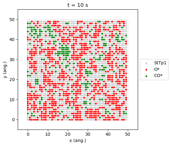
pyZacros also offers some predefined plot functions that use matplotlib as well. For example, it is possible to see a typical reactive state configuration $x_\text{CO}=0.54$ and one in the process of being poisoned by $CO$ ($x_\text{CO}=0.55$). Just get the last lattice state with the last_lattice_state() function and visualize it with plot(). See the code and figures below.

The state at $x_\text{CO}=0.54$ is a prototypical steady-state,

results[33].last_lattice_state().plot()

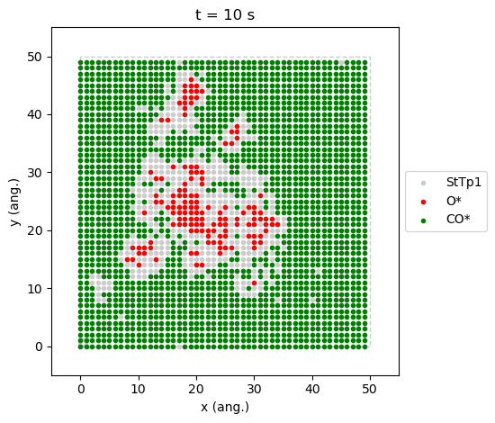
contrary to the one at $x_\text{CO}=0.55$, is a good example where we can see the two phases coexisting.

results[34].last_lattice_state().plot()

In the previous paragraph, we introduced the concept of steady-state. However, let’s define it slightly more formally. For our study system, the steady-state for a given composition is characterized when the derivative of the $CO_2$ production (TOF) with respect to time is zero and remains so:

\[\frac{d}{dt}TOF_{\text{CO}_2} = 0, \,\,\text{for all present and future}\,\, t\]

pyZacros also offers the function plot_molecule_numbers() to visualize the molecule numbers and its first derivative as a function of time. See code and figures below:

results[33].plot_molecule_numbers( ["CO2"], normalize_per_site=True )
results[34].plot_molecule_numbers( ["CO2"], normalize_per_site=True )

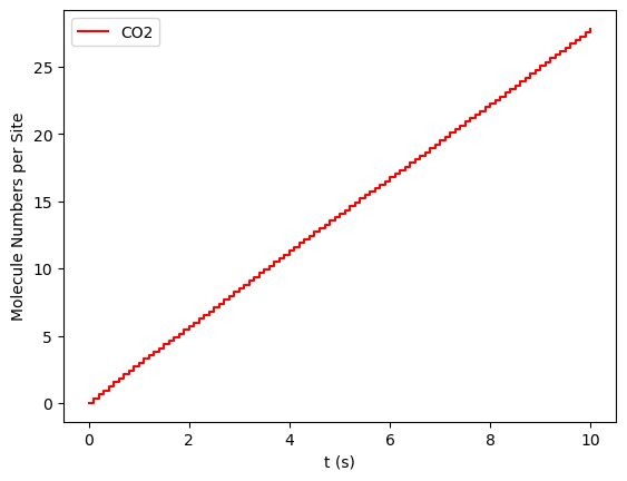
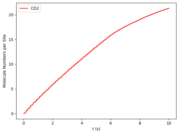
results[33].plot_molecule_numbers( ["CO2"], normalize_per_site=True, derivative=True )
results[34].plot_molecule_numbers( ["CO2"], normalize_per_site=True, derivative=True )

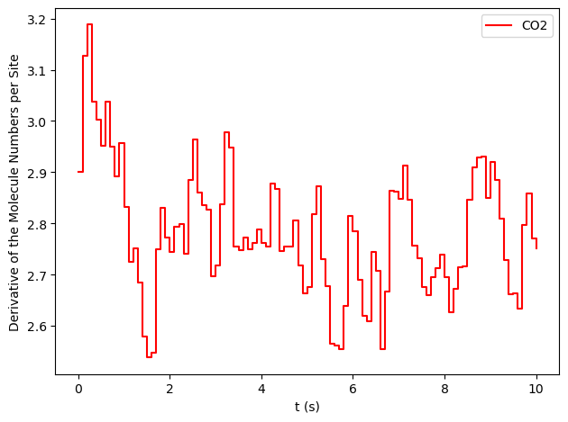
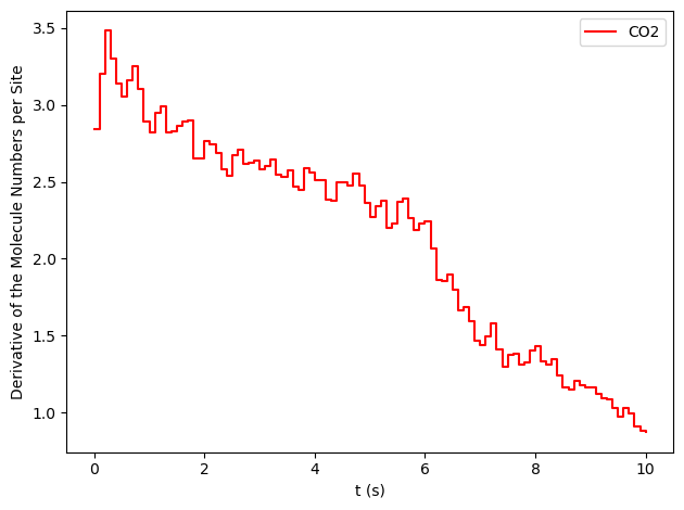
From the figures above, it is clear that we have reached a steady-state for $x_\text{CO}=0.54$. Notice that the first derivative is approximately constant at 2.7 mol/s/site within a tolerance of 5 mol/s/site. Contrary, this is not the case of $x_\text{CO}=0.55$, where the first derivative continuously decreases.

Now, we can close the pyZacros environment:

scm.pyzacros.finish()

[02.02|22:24:09] PLAMS run finished. Goodbye

As a final note, you can use the following script to visualize the results by loading them directly from disk rather than running the entire calculation.

import scm.pyzacros as pz

# xCO=0.54
job = pz.ZacrosJob.load_external( path="plams_workdir/plamsjob.034" )
job.results.last_lattice_state().plot()
job.results.plot_molecule_numbers( ["CO2"], normalize_per_site=True )
job.results.plot_molecule_numbers( ["CO2"], normalize_per_site=True, derivative=True )

# xCO=0.55
job = pz.ZacrosJob.load_external( path="plams_workdir/plamsjob.035" )
job.results.last_lattice_state().plot()
job.results.plot_molecule_numbers( ["CO2"], normalize_per_site=True )
job.results.plot_molecule_numbers( ["CO2"], normalize_per_site=True, derivative=True )

Note

The code described in this tutorial that allows defining the system can be significantly reduced using the ZiffGulariBarshad predefined model in pyZacros as follows:

import scm.pyzacros.models
zgb = pz.models.ZiffGulariBarshad()

Then you can access its properties using zgb.lattice, zgb.mechanism, and zgb.cluster_expansion.

Additionally, the code taking care of individual executions of the ZacrosJob objects and recovering the results for each condition can also be simplified by using the Extended Component ZacrosParametersScanJob.

Take a look at the example PhaseTransitions-v2.py for further details. It reproduces the results of this tutorial but using the predefined models and the extended components.