Ziff-Gulari-Barshad Model: Steady State Conditions
Note
To follow this tutorial, either:
Download
SteadyState.py(run as$AMSBIN/amspython SteadyState.py).Download
SteadyState.ipynb(see also: how to install Jupyterlab)
The mechanism being studied frequently involves several intermediary
species, which concentrations (partial pressure for species in the gas
phase and coverage fraction for species that are adsorbed) change in a
particular manner as the simulation progresses. However, after a
particular simulation time, the concentration of all intermediate
species remains constant. At that point, we say the system has reached a
steady state configuration. Sadly, we are unable to anticipate the
simulation time at which that stage will be reached. Therefore, the more
logical approach to take is to: 1) run the simulation for a set period
of time (initial guess), 2) determine if the system has reached a steady
state, and 3) if so, consider the calculation to have converged and
stop; otherwise, increase the simulation time and resume repeating all
steps until convergence. With pyZacros, and much more directly with
Zacros, this is laborious to complete manually. Thus, this tutorial
aims to demonstrate how to accomplish this goal using the class
ZacrosSteadyStateJob from the pyZacros extended components.
The first step is to import all packages we need:
import numpy
import scm.pyzacros as pz
import scm.pyzacros.models
Then, we initialize the pyZacros environment.
scm.pyzacros.init()
PLAMS working folder: /home/user/pyzacros/examples/ZiffGulariBarshad/plams_workdir
Notice this command created the directory where all Zacros input and
output files will be stored if they are needed for future reference
(plams_workdir by default). Typically, the user doesn’t need to use
these files.
First, we define the physical system to study. Here we used the Ziff-Gulari-Bashard model. This simple model describes the catalytic processes of carbon monoxide oxidation to carbon dioxide (\(\text{CO}+\frac{1}{2}\text{O}_2\longrightarrow \text{CO}_2\)) and accurately captures the interesting property of the phase transition between two surface poisoned states (either CO- or O-poisoned) and a steady state in between. It is named after Robert M. Ziff, Erdogan Gulari, and Yoav Barshad’s pioneering work in 1986. Check the API documentation for more details about its implementation in pyZacros.
zgb = pz.models.ZiffGulariBarshad()
Then, we set up the Zacros calculation. All parameters are set using a
Setting object. To begin, we define the physical parameters: the
molar fractions of the gas species (CO and O2), the temperature
(in K), and the pressure (in bar). The calculation parameters are then
set: species numbers (in s) determines how frequently information
about the number of gas and surface species will be stored, max time
(in s) specifies the maximum allowed simulated time, and “random seed”
specifies the random seed to make the calculation precisely
reproducible. Keep in mind that max time defines the calculation’s
stopping criterion, and it is the parameter we will control below to
achieve the steady-state configuration. Finally, we create the
ZacrosJob, which uses the parameters we just defined as well as the
Ziff-Gulari-Bashard model’s lattice, mechanism, and cluster expansion.
Notice we do not run this job, we use it as a reference for the
steady-state calculation described below.
z_sett = pz.Settings()
z_sett.molar_fraction.CO = 0.42
z_sett.molar_fraction.O2 = 1.0 - z_sett.molar_fraction.CO
z_sett.temperature = 500.0
z_sett.pressure = 1.0
z_sett.species_numbers = ("time", 0.1)
z_sett.max_time = 100.0 * 0.1
z_sett.random_seed = 953129

job = pz.ZacrosJob(
    settings=z_sett, lattice=zgb.lattice, mechanism=zgb.mechanism, cluster_expansion=zgb.cluster_expansion
)
It is now time to set up the steady state calculation. It also needs a
Settings object to set its parameters, as shown in the first block
of code below. To begin, we define the parameters for calculating the
turn-over frequency (TOF), which is the property that will be monitored
to determine convergence as the steady state is reached. In a nutshell,
for a given simulation time (that will be increased systematically), the
simulation is divided into an turnover_frequency.nbatch ensemble of
contiguous batches (20 for this case) where the TOFs are calculated for
each one. If the estimated confidence level for these TOFs is higher
than the confidence level specified by the
turnover frequency.confidence parameter (96% for this case),
convergence is then considered to have been achieved. The
turnover frequency.nreplicas parameter allows several simulations to
run in parallel to speed up the calculation at the expense of more
computational power. For the time being, we will leave it at 1, but we
will return to it later.
In the second block of code, the ZacrosSteadyStateJob.Parameters()
class allows us to specify the grid in max time, which in this case
ranges from 20 to 1000 every 100 seconds. Take note that the convergence
is verified for each point on this grid, and if it has not converged,
the calculation is resumed up to the next point in max time.
Finally, we create ZacrosSteadyStateJob, which references the
ZacrosJob defined above as well as the Settings object and
parameters we just defined:
ss_sett = pz.Settings()
ss_sett.turnover_frequency.nbatch = 20
ss_sett.turnover_frequency.confidence = 0.96
ss_sett.turnover_frequency.nreplicas = 1

parameters = pz.ZacrosSteadyStateJob.Parameters()
parameters.add("max_time", "restart.max_time", numpy.arange(20.0, 1000.0, 100))

ss_job = pz.ZacrosSteadyStateJob(settings=ss_sett, reference=job, parameters=parameters)
[27.01|09:11:22] JOB plamsjob Steady State Convergence: Using nbatch=20,confidence=0.96,ignore_nbatch=1,nreplicas=1
The steady-state calculation setup is ready. Therefore, we can start it
by invoking the function run(), which will provide access to the
results via the results variable after it has been completed. The
sentence involving the method ok(), verifies that the calculation
was successfully executed, and waits for the completion of every
executed thread in case of parallel execution.
results = ss_job.run()

if not ss_job.ok():
    print("Something went wrong!")
[27.01|09:11:22] JOB plamsjob STARTED
[27.01|09:11:22] JOB plamsjob RUNNING
[27.01|09:11:22] JOB plamsjob/ss_iter000 Steady State: NEW
[27.01|09:11:22] JOB plamsjob/ss_iter000 STARTED
[27.01|09:11:22] JOB plamsjob/ss_iter000 RUNNING
[27.01|09:11:22] JOB plamsjob/ss_iter000 FINISHED
[27.01|09:11:23] JOB plamsjob/ss_iter000 SUCCESSFUL
[27.01|09:11:23]       species            TOF          error          ratio     conv?
[27.01|09:11:23]            CO       -0.57600        0.08915        0.15478     False
[27.01|09:11:23]            O2       -0.29120        0.07190        0.24691     False
[27.01|09:11:23]           CO2        0.57667        0.08573        0.14866     False
[27.01|09:11:23] JOB plamsjob Steady State Convergence: NO CONVERGENCE REACHED YET
[27.01|09:11:23] JOB plamsjob/ss_iter001 Steady State: NEW (dep=plamsjob/ss_iter000)

...

[27.01|09:11:44] JOB plamsjob/ss_iter007 FINISHED
[27.01|09:11:45] JOB plamsjob/ss_iter007 SUCCESSFUL
[27.01|09:11:46]       species            TOF          error          ratio     conv?
[27.01|09:11:46]            CO       -0.60170        0.02183        0.03628      True
[27.01|09:11:46]            O2       -0.30081        0.01095        0.03639      True
[27.01|09:11:46]           CO2        0.60170        0.02183        0.03628      True
[27.01|09:11:46] JOB plamsjob Steady State Convergence: CONVERGENCE REACHED. DONE!
[27.01|09:11:46] JOB plamsjob FINISHED
[27.01|09:11:47] JOB plamsjob SUCCESSFUL
If the execution got up to this point, everything worked as expected. Hooray!
Now, in the following lines, we just nicely print the results in a
table. See the API documentation to learn more about how the results
object is structured. Here we show the history of the simulation and see
how it progresses as the max_time is increased. We print the TOF for
CO2 (in mol/s/site), its error, and whether the calculation converged.
Notice that the calculation should have been converged at 720 s of
max_time.
print(60 * "-")
fline = "{0:>8s}{1:>10s}{2:>15s}{3:>12s}{4:>10s}"
print(fline.format("iter", "max_time", "TOF_CO2", "error", "conv?"))
print(60 * "-")

for i, step in enumerate(results.history()):
    fline = "{0:8d}{1:>10.2f}{2:15.5f}{3:>12.5f}{4:>10s}"
    print(
        fline.format(
            i,
            step["max_time"],
            step["turnover_frequency"]["CO2"],
            step["turnover_frequency_error"]["CO2"],
            str(all(step["converged"].values())),
        )
    )
------------------------------------------------------------
    iter  max_time        TOF_CO2       error     conv?
------------------------------------------------------------
       0     20.00        0.57667     0.08573     False
       1    120.00        0.59301     0.03157     False
       2    220.00        0.59360     0.03311     False
       3    320.00        0.59293     0.03062     False
       4    420.00        0.59345     0.02729     False
       5    520.00        0.61241     0.02564     False
       6    620.00        0.60345     0.02697     False
       7    720.00        0.60170     0.02183      True
Now that all calculations are done, we can close the pyZacros environment:
scm.pyzacros.finish()
[27.01|09:11:47] PLAMS run finished. Goodbye
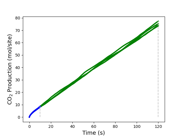
Additionally, you can see the aforementioned results visually if you have installed the package matplotlib. Please review the code below. In particular, pay close attention to how to obtain the “children results” (each thread executed) which are identified by their replica and iteration number. In the figure, each iteration is represented by a different color, and the stopping points on “max time” are represented by vertical gray dashed lines.
import matplotlib.pyplot as plt

fig = plt.figure()
ax = plt.axes()
ax.set_xlabel("Time (s)", fontsize=14)
ax.set_ylabel("CO$_2$ Production (mol/site)", fontsize=14)

colors = "bgrcmykb"
for i in range(results.niterations()):
    for j in range(results.nreplicas()):
        molecule_numbers = results.children_results(i, j).molecule_numbers(["CO2"], normalize_per_site=True)

        ax.plot(molecule_numbers["Time"], molecule_numbers["CO2"], lw=3, color=colors[i], zorder=-i)
        ax.vlines(
            max(molecule_numbers["Time"]),
            0,
            max(molecule_numbers["CO2"]),
            colors="0.8",
            linestyles="--",
        )

plt.show()

Using Replicas
In the example script, we can increase the number of replicas in order to parallelize the steady-state search. We will use 4 replicas here:
1ss_sett.turnover_frequency.nreplicas = 4
If we run the script again, we will see that the simulation converges much faster:
The calculation now only takes two iterations, rather than the previous eight. Each replica performs a calculation with a different random seed, thereby sampling a different set of states. The TOFs for each iteration are taken as the average over the replicas. This reduces the TOF variance and accelerates the convergence by increasing the number of samples that is generated in each iteration.