Langmuir-Hinshelwood Model: Acceleration by Automated Rescaling of the Rate Constants
Note
To follow this tutorial, either:
Download
CoveragesAndReactionRate.py(run as$AMSBIN/amspython CoveragesAndReactionRate.py).Download
CoveragesAndReactionRate.ipynb(see also: how to install Jupyterlab)
The scale disparity issue is common in Kinetic Monte Carlo simulations. It emerges as a result of the fact that some fundamental events or groups of them typically occur at vastly different time scales; in other words, their rate constants can span multiple orders of magnitude. In heterogeneous catalysis, there are typically two groups: 1) very fast events that correspond to the species’ surface diffusions and 2) slow reactions that change their chemical identity. The latter group of events is usually the one of interest because it allows the evaluation of the material’s catalytic activity. In contrast, the species’ surface diffusion does not contribute significantly to the net evolution of the slow reactions. But, as becomes the most frequent step, it also becomes the limiting factor of the simulation progress, considerably increasing the computational cost. This tutorial shows how to speed up the calculation by several orders of magnitude without sacrificing precision by automatically detecting and scaling the rate constants of fast reactions.
We will focus on the net reaction \(\text{CO}+\frac{1}{2}\text{O}_2\longrightarrow \text{CO}_2\) that takes place at a catalyst’s surface and whose reaction mechanism is described by the Langmuir-Hinshelwood model. Because this model has four very fast processes (\(CO\) and \(O_2\) adsorption, and \(O*\) and \(CO*\) diffusion) and one slow process (\(CO\) oxidation), it is an ideal prototype for demonstrating the benefits of the automated rescaling of rate constants technique. Our ultimate goal is to investigate how altering the relative percentage of the gas reactants \(CO\) and \(O_2\) (at a specific temperature and pressure) affect the rate of \(CO_2\) production under steady state conditions. This example is inspired on Zacros tutorial What’s KMC All About and Why Bother.
Let’s start! The first step is to import all packages we need:
import multiprocessing
import numpy
import scm.plams
import scm.pyzacros as pz
import scm.pyzacros.models
Then, we initialize the pyZacros environment.
scm.pyzacros.init()
PLAMS working folder: /home/user/pyzacros/examples/ZiffGulariBarshad/plams_workdir
Notice this command created the directory where all Zacros input and
output files will be stored if they are needed for future reference
(plams_workdir by default). Typically, the user doesn’t need to use
these files.
This calculation necessitates a significant computational effort. On a
typical laptop, it should take around 20 min to complete. So, in order
to speed things up, we’ll use the plams.JobRunner class to run as
many parallel instances as possible. In this case, we choose to use the
maximum number of simultaneous processes (maxjobs) equal to the
number of processors in the machine.
maxjobs = multiprocessing.cpu_count()
scm.plams.config.default_jobrunner = scm.plams.JobRunner(parallel=True, maxjobs=maxjobs)
print("Running up to {} jobs in parallel simultaneously".format(maxjobs))
Running up to 8 jobs in parallel simultaneously
First, we initialize our Langmuir-Hinshelwood model, which by luck is available as a predefined model in pyZacros,
lh = pz.models.LangmuirHinshelwood()
Then, we must set up a ZacrosParametersScanJob calculation, which
will allow us to scan the molar fraction of \(CO\) as a parameter.
However, this calculation requires the definition of a
ZacrosSteadyStateJob, that in turns requires a ZacrosJob. So, We
will go through them one at a time:
1. Setting up the ZacrosJob
For ZacrosJob, all parameters are set using a Setting object. To
begin, we define the physical parameters: temperature (in K), and
pressure (in bar). The calculation parameters are then set:
species numbers (in s) determines how frequently information about
the number of gas and surface species will be stored, max time (in
s) specifies the maximum allowed simulated time, and “random seed”
specifies the random seed to make the calculation precisely
reproducible. Keep in mind that max time defines the calculation’s
stopping criterion, and it is the parameter that will be controlled
later to achieve the steady-state configuration. Finally, we create the
ZacrosJob, which uses the parameters we just defined as well as the
Langmuir-Hinshelwood model’s lattice, mechanism, and cluster expansion.
Notice we do not run this job, we use it as a reference for the
steady-state calculation described below.
z_sett = pz.Settings()
z_sett.temperature = 500.0
z_sett.pressure = 1.000
z_sett.species_numbers = ("time", 1.0e-5)
z_sett.max_time = 100 * 1.0e-5
z_sett.random_seed = 1609

z_job = pz.ZacrosJob(
    settings=z_sett, lattice=lh.lattice, mechanism=lh.mechanism, cluster_expansion=lh.cluster_expansion
)
2. Setting up the ZacrosSteadyStateJob
We also need to create a Setting object for ZacrosJob There, we
ask for a steady-state configuration using a TOFs calculation with a 95%
confidence level (turnover frequency.confidence), using four
replicas to speed up the calculation (turnover frequency.nreplicas);
for more information, see example Ziff-Gulari-Barshad model: Steady
State Conditions. Then, we ask for the rate constants to be
automatically scaled (scaling.enabled) using an inspection time of
0.0006 s (“scaling.max time”). In a nutshell, the scaling algorithm uses
this maximum time and the original rate constants to execute a probe
simulation. From there, the occurrence rates for each reaction are
determined and scaled appropriately. Only reactions that are proven to
be quasi-equilibrated are modified. The actual simulation is then
started from the beginning using the new reaction rates following this.
The ZacrosSteadyStateJob.Parameters object allows to set the grid of
maximum times to explore in order to reach the steady state
(ss_params). Finally, we create ZacrosSteadyStateJob, which
references the ZacrosJob defined above (z_job) as well as the
Settings object and parameters we just defined:
ss_sett = pz.Settings()
ss_sett.turnover_frequency.confidence = 0.95
ss_sett.turnover_frequency.nreplicas = 4
ss_sett.scaling.enabled = "T"
ss_sett.scaling.max_time = 60 * 1e-5

ss_params = pz.ZacrosSteadyStateJob.Parameters()
ss_params.add("max_time", "restart.max_time", 2 * z_sett.max_time * (numpy.arange(10) + 1) ** 2)

ss_job = pz.ZacrosSteadyStateJob(settings=ss_sett, reference=z_job, parameters=ss_params)
[27.01|09:15:05] JOB plamsjob Steady State Convergence: Using nbatch=20,confidence=0.95,ignore_nbatch=1,nreplicas=4
3. Setting up the ZacrosParametersScanJob
Although the ZacrosParametersScanJob does not require a Setting
object, it does require a ZacrosSteadyStateJob.Parameters object to
specify which parameters must be modified systematically. In this
instance, all we need is a dependent parameter, the \(O_2\) molar
fraction x_O2, and an independent parameter, the \(CO\) molar
fraction x_CO, which ranges from 0.05 to 0.95. Keep in mind that the
condition x_CO+x_O2=1 must be met. These molar fractions will be
used internally to replace molar fraction.CO and
molar fraction.O2 in the Zacros input files. Then, using the
ZacrosSteadyStateJob defined earlier (ss job) and the parameters
we just defined (ps params), we create the
ZacrosParametersScanJob:
ps_params = pz.ZacrosParametersScanJob.Parameters()
ps_params.add("x_CO", "molar_fraction.CO", numpy.linspace(0.05, 0.95, 11))
ps_params.add("x_O2", "molar_fraction.O2", lambda params: 1.0 - params["x_CO"])

ps_job = pz.ZacrosParametersScanJob(reference=ss_job, parameters=ps_params)
[27.01|09:15:05] JOB ps_cond000 Steady State Convergence: Using nbatch=20,confidence=0.95,ignore_nbatch=1,nreplicas=4
[27.01|09:15:05] JOB ps_cond001 Steady State Convergence: Using nbatch=20,confidence=0.95,ignore_nbatch=1,nreplicas=4
[27.01|09:15:05] JOB ps_cond002 Steady State Convergence: Using nbatch=20,confidence=0.95,ignore_nbatch=1,nreplicas=4
[27.01|09:15:05] JOB ps_cond003 Steady State Convergence: Using nbatch=20,confidence=0.95,ignore_nbatch=1,nreplicas=4
[27.01|09:15:05] JOB ps_cond004 Steady State Convergence: Using nbatch=20,confidence=0.95,ignore_nbatch=1,nreplicas=4
[27.01|09:15:05] JOB ps_cond005 Steady State Convergence: Using nbatch=20,confidence=0.95,ignore_nbatch=1,nreplicas=4
[27.01|09:15:05] JOB ps_cond006 Steady State Convergence: Using nbatch=20,confidence=0.95,ignore_nbatch=1,nreplicas=4
[27.01|09:15:05] JOB ps_cond007 Steady State Convergence: Using nbatch=20,confidence=0.95,ignore_nbatch=1,nreplicas=4
[27.01|09:15:05] JOB ps_cond008 Steady State Convergence: Using nbatch=20,confidence=0.95,ignore_nbatch=1,nreplicas=4
[27.01|09:15:05] JOB ps_cond009 Steady State Convergence: Using nbatch=20,confidence=0.95,ignore_nbatch=1,nreplicas=4
[27.01|09:15:05] JOB ps_cond010 Steady State Convergence: Using nbatch=20,confidence=0.95,ignore_nbatch=1,nreplicas=4
The parameters scan calculation setup is ready. Therefore, we can start
it by invoking the function run(), which will provide access to the
results via the results variable after it has been completed. The
sentence involving the method ok(), verifies that the calculation
was successfully executed, and waits for the completion of every
executed thread. Go and grab a cup of coffee, this step will take around
15 mins!
results = ps_job.run()

if not ps_job.ok():
    print("Something went wrong!")
[27.01|09:15:05] JOB plamsjob STARTED
[27.01|09:15:05] Waiting for job plamsjob to finish
[27.01|09:15:05] JOB plamsjob RUNNING
[27.01|09:15:05] JOB plamsjob/ps_cond000 STARTED
[27.01|09:15:05] JOB plamsjob/ps_cond001 STARTED
[27.01|09:15:05] JOB plamsjob/ps_cond002 STARTED

...

[27.01|09:31:03]       species            TOF          error          ratio     conv?
[27.01|09:31:03]            CO      -52.52688        4.84537        0.09225     False
[27.01|09:31:03]            O2      -26.90450        2.78063        0.10335     False
[27.01|09:31:03]           CO2       52.91640        4.65244        0.08792     False
[27.01|09:31:03]    Replica #2
[27.01|09:31:03]       species            TOF          error          ratio     conv?
[27.01|09:31:04]            CO     -225.40015       12.98476        0.05761     False
[27.01|09:31:04]            O2     -115.66183        4.44209        0.03841      True
[27.01|09:31:04]           CO2      228.95111        8.73665        0.03816      True
[27.01|09:31:04]    Average
[27.01|09:31:04]       species            TOF          error          ratio     conv?
[27.01|09:31:04]            CO      -54.87733        1.63967        0.02988      True
[27.01|09:31:04]            O2      -26.85096        1.08631        0.04046      True
[27.01|09:31:04]           CO2       54.73375        1.56100        0.02852      True
[27.01|09:31:04] JOB plamsjob/ps_cond000 Steady State Convergence: CONVERGENCE REACHED. DONE!
[27.01|09:31:04] JOB plamsjob/ps_cond000 FINISHED
[27.01|09:31:05]    Replica #3
[27.01|09:31:05]       species            TOF          error          ratio     conv?
[27.01|09:31:05]            CO     -216.58663       13.48940        0.06228     False
[27.01|09:31:05]            O2     -106.99160        5.19478        0.04855      True
[27.01|09:31:05]           CO2      214.75940       10.88629        0.05069     False
[27.01|09:31:06]    Average
[27.01|09:31:06]       species            TOF          error          ratio     conv?
[27.01|09:31:06]            CO     -221.49798        5.07706        0.02292      True
[27.01|09:31:06]            O2     -110.17810        2.42785        0.02204      True
[27.01|09:31:06]           CO2      220.65690        4.39982        0.01994      True
[27.01|09:31:06] JOB plamsjob/ps_cond010 Steady State Convergence: CONVERGENCE REACHED. DONE!
[27.01|09:31:06] JOB plamsjob/ps_cond010 FINISHED
[27.01|09:31:06] JOB plamsjob/ps_cond000 SUCCESSFUL
[27.01|09:31:07] JOB plamsjob/ps_cond010 SUCCESSFUL
[27.01|09:31:11] JOB plamsjob FINISHED
[27.01|09:31:15] JOB plamsjob SUCCESSFUL
If the execution got up to this point, everything worked as expected. Hooray!
Finally, in the following lines, we just nicely print the results in a
table. See the API documentation to learn more about how the results
object is structured, and the available methods. In this case, we use
the turnover_frequency() and average_coverage() methods to get
the TOF for the gas species and average coverage for the surface
species, respectively. Regarding the latter one, we use the last ten
steps in the simulation to calculate the average coverages.
x_CO = []
ac_O = []
ac_CO = []
TOF_CO2 = []

results_dict = results.turnover_frequency()
results_dict = results.average_coverage(last=10, update=results_dict)

for i in range(len(results_dict)):
    x_CO.append(results_dict[i]["x_CO"])
    ac_O.append(results_dict[i]["average_coverage"]["O*"])
    ac_CO.append(results_dict[i]["average_coverage"]["CO*"])
    TOF_CO2.append(results_dict[i]["turnover_frequency"]["CO2"])

print("------------------------------------------------")
print("%4s" % "cond", "%8s" % "x_CO", "%10s" % "ac_O", "%10s" % "ac_CO", "%12s" % "TOF_CO2")
print("------------------------------------------------")
for i in range(len(x_CO)):
    print("%4d" % i, "%8.2f" % x_CO[i], "%10.6f" % ac_O[i], "%10.6f" % ac_CO[i], "%12.6f" % TOF_CO2[i])
------------------------------------------------
cond     x_CO       ac_O      ac_CO      TOF_CO2
------------------------------------------------
   0     0.05   0.665594   0.028219    54.733748
   1     0.14   0.615375   0.082844   135.299544
   2     0.23   0.582250   0.126594   198.215992
   3     0.32   0.532375   0.178719   257.936395
   4     0.41   0.497031   0.221625   300.382949
   5     0.50   0.442750   0.272969   329.214754
   6     0.59   0.402031   0.318562   352.259276
   7     0.68   0.351687   0.372437   351.805662
   8     0.77   0.297906   0.422687   332.247334
   9     0.86   0.232156   0.488156   310.444388
  10     0.95   0.144281   0.554344   220.656898
The results table above demonstrates that when \(CO\) coverage rises, the net \(CO\) oxidation reaction tends to progress more quickly until it reaches a maximum of about 0.7. At this point, it begins to decline. Notice that the maximal \(CO_2\) generation occurs simultaneously as the \(CO*\) coverage reaches parity with the \(O*\) coverage. This makes intuitive sense since, at that point, we maximize the likelihood of discovering an \(O*\) and a \(CO*\) that are close enough to react in accordance with the proper reaction’s stoichiometry. The number of \(O*\) or \(CO*\) observers rises as we move away from that critical point, decreasing the likelihood that the \(CO\) oxidation process could take place.
Now, we can close the pyZacros environment:
scm.pyzacros.finish()
[27.01|09:31:31] PLAMS run finished. Goodbye
Comparing with Traditional Kinetic Models
Note
To follow the second part of this tutorial, either:
Download
CoveragesAndReactionRate_ViewResults.py(run as$AMSBIN/amspython CoveragesAndReactionRate.py).Download
CoveragesAndReactionRate_ViewResults.ipynb(see also: how to install Jupyterlab)
The goal of this second part of the tutorial is to demonstrate how to
resume the calculation from the first part and visualize the results. In
addition, we will compare these results to an analytical model to assess
their quality. Before we begin, make sure we have the working directory
generated by CoverageAndReactionRate.ipynb or
CoverageAndReactionRate.py. We’ll assume it’s called
plams_workdir, which is the default value. However, keep in mind
that each time you run any of the above scripts, PLAMS will create a new
working directory by appending a sequential number to its name, for
example, plams_workdir.001. If this is the case, simply replace
plams_workdir with the appropriate value.
So, let’s get started!
First, we load the required packages and retrieve the
ZacrosParametersScanJob (job) and corresponding results object
(results) from the working directory, as shown below:
import scm.pyzacros as pz
import scm.pyzacros.models

scm.pyzacros.init()

job = scm.pyzacros.load("plams_workdir/plamsjob/plamsjob.dill")
results = job.results

scm.pyzacros.finish()
PLAMS working folder: /home/user/pyzacros/examples/ZiffGulariBarshad/plams_workdir.002
[27.01|09:45:00] PLAMS run finished. Goodbye
To be certain, we generate and print the same summary table from the end of the first part of the tutorial. They must be exactly the same:
x_CO = []
ac_O = []
ac_CO = []
TOF_CO2 = []

results_dict = results.turnover_frequency()
results_dict = results.average_coverage(last=10, update=results_dict)

for i in range(len(results_dict)):
    x_CO.append(results_dict[i]["x_CO"])
    ac_O.append(results_dict[i]["average_coverage"]["O*"])
    ac_CO.append(results_dict[i]["average_coverage"]["CO*"])
    TOF_CO2.append(results_dict[i]["turnover_frequency"]["CO2"])

print("------------------------------------------------")
print("%4s" % "cond", "%8s" % "x_CO", "%10s" % "ac_O", "%10s" % "ac_CO", "%12s" % "TOF_CO2")
print("------------------------------------------------")
for i in range(len(x_CO)):
    print("%4d" % i, "%8.2f" % x_CO[i], "%10.6f" % ac_O[i], "%10.6f" % ac_CO[i], "%12.6f" % TOF_CO2[i])
------------------------------------------------
cond     x_CO       ac_O      ac_CO      TOF_CO2
------------------------------------------------
   0     0.05   0.665594   0.028219    54.733748
   1     0.14   0.615375   0.082844   135.299544
   2     0.23   0.582250   0.126594   198.215992
   3     0.32   0.532375   0.178719   257.936395
   4     0.41   0.497031   0.221625   300.382949
   5     0.50   0.442750   0.272969   329.214754
   6     0.59   0.402031   0.318562   352.259276
   7     0.68   0.351687   0.372437   351.805662
   8     0.77   0.297906   0.422687   332.247334
   9     0.86   0.232156   0.488156   310.444388
  10     0.95   0.144281   0.554344   220.656898
Additionally, you can see the aforementioned results visually if you have installed the package matplotlib. Please review the code below.
import matplotlib.pyplot as plt

fig = plt.figure()

ax = plt.axes()
ax.set_xlim([0.0, 1.0])
ax.set_xlabel("Molar Fraction CO", fontsize=14)
ax.set_ylabel("Coverage Fraction (%)", color="blue", fontsize=14)
ax.plot(x_CO, ac_O, marker="$\u25CF$", color="blue", linestyle="-.", markersize=4, zorder=2)
ax.plot(x_CO, ac_CO, marker="$\u25EF$", color="blue", markersize=4, zorder=4)
plt.text(0.3, 0.60, "O*", fontsize=18, color="blue")
plt.text(0.7, 0.45, "CO*", fontsize=18, color="blue")

ax2 = ax.twinx()
ax2.set_ylabel("TOF (mol/s/site)", color="red", fontsize=14)
ax2.plot(x_CO, TOF_CO2, marker="$\u25EF$", color="red", markersize=4, zorder=6)
plt.text(0.3, 200.0, "CO$_2$", fontsize=18, color="red")

plt.show()
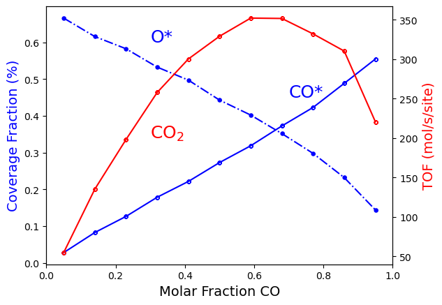
Starting from the left side of the figure, it shows that by increasing
the x_CO; the net \(CO\) oxidation reaction tends to progress
more quickly (like a first-order reaction). Then the reaction rate peaks
at around x_CO=0.7, becoming almost independent of x_CO (like a
zero-order reaction). And finally, it then begins to decline (like a
negative-order reaction). Furthermore, we can see that as we increase
the coverage of \(CO*\), we decrease the coverage of \(O*\). As
a result, when we mostly cover the surface with one of the reactants
(either \(CO*\) or \(O*\)), the rate of \(CO_2\) production
becomes slow because there isn’t enough of the complementary reactant on
the surface. So, it is not a surprise, that the maximum \(CO_2\)
generation coincides with the point at which \(CO*\) coverage equals
\(O*\) coverage.
In the Zacros tutorial What’s KMC All About and Why Bother?, there is a thorough discussion of Langmuir-Hinshelwood-type models, their approximations with respect to a real system, and how to obtain analytical expressions for reactant coverages and the net reaction rates concerning gas phase composition. In particular, these expressions are reached by making the fundamental assumption that both diffusion and adsorption/desorption events are quasi-equilibrated (being the later one the rate-limiting factor), occurring on a much faster timescale than the oxidation event. We use the same argument to speed up our calculations. Thus, we can use the analytical expressions we obtained to assess the overall quality of our results. Our results should be indistinguishable from the Langmuir-Hinshelwood deterministic equations, which are shown below:
Here \(B_\text{CO}\)/\(B_{\text{O}_2}\) represent the ratio of
the adsorption-desorption pre-exponential terms of
\(CO\)/\(O_2\) (pe_ratio in Zacros),
\(x_\text{CO}\)/\(x_{\text{O}_2}\) the molar fractions of
\(CO\)/\(O_2\); \(\theta_\text{CO}\)/\(\theta_\text{O}\)
the coverage of \(CO*\)/\(O*\), \(A_\text{oxi}\) the
pre-exponential factor of the CO oxidation step (pre_expon in
Zacros), and TOF\(_{\text{CO}_2}\) the turnover frequency or
production rate of \(CO_2\). The number 6 is because, in our
lattice, each site has 6 neighbors, so the oxidation event is
“replicated” across each neighboring site.
Notice that to get the above expressions based on the ones shown in the Zacros tutorial, you need the following equalities:
The final equality follows from the fact that in pyZacros, the activation energy for all elementary reactions is equal to zero.
The code below simply computes the coverages and TOF of \(CO_2\) using the analytical expression described above:
import numpy

lh = pz.models.LangmuirHinshelwood()

B_CO = lh.mechanism.find_one("CO_adsorption").pe_ratio
B_O2 = lh.mechanism.find_one("O2_adsorption").pe_ratio
A_oxi = lh.mechanism.find_one("CO_oxidation").pre_expon

x_CO_model = numpy.linspace(0.0, 1.0, 201)

ac_O_model = []
ac_CO_model = []
TOF_CO2_model = []

for i in range(len(x_CO_model)):
    x_O2 = 1 - x_CO_model[i]
    ac_O_model.append(numpy.sqrt(B_O2 * x_O2) / (1 + B_CO * x_CO_model[i] + numpy.sqrt(B_O2 * x_O2)))
    ac_CO_model.append(B_CO * x_CO_model[i] / (1 + B_CO * x_CO_model[i] + numpy.sqrt(B_O2 * x_O2)))
    TOF_CO2_model.append(6 * A_oxi * ac_CO_model[i] * ac_O_model[i])
Additionally, if you have installed the package matplotlib, you can see the aforementioned results visually. Please look over the code below, and notice we plot the analytical and simulation results together. The points in the figure represent simulation results, while the lines represent analytical model results. They are nearly identical.
import matplotlib.pyplot as plt

x_CO_max = (B_O2 / B_CO**2 / 2.0) * (numpy.sqrt(1.0 + 4.0 * B_CO**2 / B_O2) - 1.0)

fig = plt.figure()

ax = plt.axes()
ax.set_xlim([0.0, 1.0])
ax.set_xlabel("Molar Fraction CO", fontsize=14)
ax.set_ylabel("Coverage Fraction (%)", color="blue", fontsize=14)
ax.vlines(x_CO_max, 0, max(ac_O_model), colors="0.8", linestyles="--")
ax.plot(x_CO_model, ac_O_model, color="blue", linestyle="-.", lw=2, zorder=1)
ax.plot(x_CO, ac_O, marker="$\u25CF$", color="blue", lw=0, markersize=4, zorder=2)
ax.plot(x_CO_model, ac_CO_model, color="blue", linestyle="-", lw=2, zorder=3)
ax.plot(x_CO, ac_CO, marker="$\u25EF$", color="blue", markersize=4, lw=0, zorder=4)
plt.text(0.3, 0.60, "O*", fontsize=18, color="blue")
plt.text(0.7, 0.45, "CO*", fontsize=18, color="blue")

ax2 = ax.twinx()
ax2.set_ylabel("TOF (mol/s/site)", color="red", fontsize=14)
ax2.plot(x_CO_model, TOF_CO2_model, color="red", linestyle="-", lw=2, zorder=5)
ax2.plot(x_CO, TOF_CO2, marker="$\u25EF$", color="red", markersize=4, lw=0, zorder=6)
plt.text(0.3, 200.0, "CO$_2$", fontsize=18, color="red")

plt.show()

As a final note, we included in the code above the value of the \(CO\) molar fraction (\(x_\text{CO}^*\)) on which we get the maximum \(CO_2\) production rate. The figure shows this value as a vertical gray dashed line. It is simple to deduce it from the preceding analytical expressions:
Notice that the position of this maximum \(x_\text{CO}*\) depends
exclusively on the ratio of the pe_ratio parameters for \(CO\)
and \(O_2\) in the Langmuir-Hinshelwood model.