Fragment Analysis¶

This tutorial will show you how to do a Fragment Analysis using ADF. The two examples used here are:

Ni(CO)₄
PtCl₄ H₂ ^2-

You will set up the calculations, run them, and visualize the results.

The first example in this tutorial is Ni(CO)₄ . It consists of one Ni fragment and once CO fragment that is repeated four times.

The second example is PtCl₄ H₂ ^2- . It consists of a PtCl₄ ^2- fragment, and one H₂ fragment. It is a good example on how to specify the charges of the fragments.

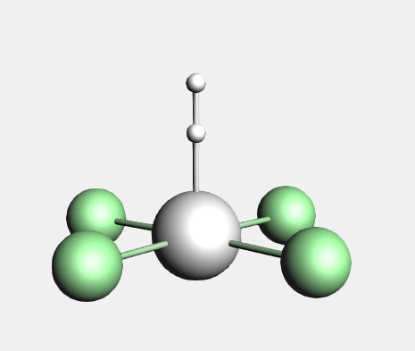
Step 1: Build Ni(CO)₄¶

The structure is perfectly tetrahedral. You should be able to build the molecule yourself, using the techniques described in earlier tutorials. One possible way:

: Start ADFinput

Build a tetrahedral metal complex: Structure Tool → Metal Complexes → ML4 tetrahedral

Change the central atom into a Ni atom

Select one ligand

Select all ligands: Select → Select Atoms Of Same Type menu command

Change them in CO ligands: Atoms → Replace By Structure → Ligands → CO

Choose the Geometry Optimization task

Save and Run

When the run has finished, click ‘Yes’ to import the optimized coordinates

Save

Or, easier, copy-paste the following coordinates:

Ni       0.35377168      -1.62413362       0.00000000
O      -1.37321951       0.10285758       1.72699119
O       2.08076287      -3.35112481       1.72699119
O      -1.37321951      -3.35112481      -1.72699119
O       2.08076287       0.10285758      -1.72699119
C       1.40953776      -0.56836754      -1.05576608
C      -0.70199440      -2.67989970      -1.05576608
C       1.40953776      -2.67989970       1.05576608
C      -0.70199440      -0.56836754       1.05576608

Your molecule should look something like this:

Step 2: Define fragments¶

The fragments that ADF uses are based on the regions that you define. In this example we will generate four new regions: one for each of the CO ligands. The regions for the CO ligands will get special names to make sure that ADF recognizes them as one fragment repeated four times.

The Ni atom will not be in a region. ADFinput will automatically create atomic fragments for all atoms not in a region.

Repeated fragments are indicated with the fragment name followed by ‘/n’, with n the number of the copy. All copies must match such that one fragment can be positioned exactly over another fragment by rotation and translation. ADF checks for this, ADFinput does not. In this particular example all four CO fragments are obviously identical by symmetry.

: Panel bar Model → Regions

Select all atoms

Click the ‘+’ button to add another new region (containing all atoms)

Select the Ni atom

Remove the Ni atom from Region_1: click the ‘-‘ button on the right side of the ‘Region_1’

Change the name of ‘Region_1’ into ‘CO’

Now one new region has been defined: the CO region for the ligands. The next step is to split the ligand region into four repeated regions:

: Press the triangle on the right side of the CO region line

In the pop-up menu, use the ‘Split By Molecule’ command

This should result in the following regions:

Step 3: set up the fragment analysis run¶

The next step is very easy: we will tell ADF to perform a Single Point calculation (fragment analysis in ADF only works with a single point calculation), and we tell ADFinput to use the regions that we just defined as fragments:

: Open the ‘Main’ panel

Select the Single Point task

Panel bar MultiLevel → Fragments

Check the ‘Use fragments’ check box

Tip

The to the right of Task links to the Fragments panel if the task is “Single Point”

In the Fragments panel you will see that one fragment is present, without charge: the repeated CO fragment. ADF will use basic atomic atoms for any atoms not put in another fragment. Thus, the Ni atom will be an atomic fragment.

Step 4: Run the fragment analysis and view the results¶

Next you will Save and Run the calculation. When you do this, ADFinput will actually save two different calculations:

The CO calculation (with matching .adf and .run file)
The Ni(CO)₄ fragment analysis calculation (with matching .adf and .run file)

You do not need to run the calculation for the CO fragment first, it will automatically be executed when needed.

: Save

Run

Observe the running of the fragment (CO), and the final fragment analysis

The CO-fragment and Ni(CO)₄ calculations all have been performed.

This calculation results in the normal .t21 and .out output files. You can view them with the SCM → View and SCM → Output commands. More interesting in the case of a fragment analysis is the interaction diagram that you can view using ADFlevels:

: SCM → Levels

In the center you see the levels of the whole molecule, on the sides you see the CO fragment and the Ni-atom fragment.

The red interaction lines tell you which molecular orbitals come from which fragment orbitals. The brightness of the line is directly related to the contribution %.

The blue interaction lines together show the orbital interaction, and are drawn when a bonding and anti-bonding combination can be made. The strength of this interaction is calculated by taking the geometric average of the 4 contributions. Compared to the normal average, the geometric average places more emphasis on equal contributions. This will give 50-50 contributions the strongest interaction, and 0-100 contributions no interaction at all. The strongest interaction is drawn, and weaker interactions can be drawn by using the menu or the shortcuts.

In the output file you can find detailed information about the composition of the molecular levels in terms of the fragment orbitals.

Step 5: Build PtCl₄ H₂ ^2-¶

We will now perform a similar fragment calculation for a PtCl₄ H₂ ^2- molecule. The following is a picture of the PtCl₄ H₂ ^2- molecule, after optimization with ADF:

To make this molecule, an easy way is to start with an octahedral complex to ensure symmetry. Next make changes to get this molecule, ending with a geometry optimization with ADF:

: Build an octahedral metal complex using the Structures button

(Structure Tool → Metal Complexes → ML6 octahedral)

Change the central atom into a Pt atom

Change four dummies in a plane into Cl atoms

Remove one of the remaining dummies

Change the remaining dummy in OH, via Structure Tool → Ligands → OH

(this will ensure the final two H’s do not break symmetry)

Change the O atom into an H atom

Choose the Geometry Optimization task

Set the total charge to -2

Select the Scalar Relativity option

Run

When the run has finished, click ‘Yes’ to import the optimized coordinates

Save

Note that pre-optimization using UFF will make the geometry worse, if you wish you can pre-optimize using Mopac. But the ADF geometry optimization will also converge without pre-optimization.

Or, copy-paste the following coordinates:

Pt       0.38536627      -1.52983373      -0.01810864
Cl       2.77381502      -1.31408830      -0.07406771
Cl       0.16595918       0.84735169      -0.25308724
Cl      -2.00032449      -1.73494925       0.12601673
H        0.29288292      -1.88628621      -2.97458718
Cl       0.60753135      -3.89638924       0.30503626
H        0.31810457      -1.78907605      -2.16830927

After copy-pasting the H atoms will not be bonded in the picture. That is no problem as ADF does only look at the atom positions.

Step 6: Define fragments¶

Define the PtCl₄ ^2- and H₂ fragments in the Regions panel:

: Panel bar Model → Regions

Select the Pt and Cl atoms

Use the ‘+’ button to add a new region, and name it ‘PtCl4’

Select the two H atoms

Use the ‘+’ button to add a new region, and name it ‘H2’

Clear the atom selection (click in empty space)

Now the fragments are defined. Next, we set up the fragment analysis calculation:

: Select ‘Main’ panel

Select the Single Point task

Panel bar MultiLevel → Fragments (or click the button)

Check the ‘Use fragments’ check box

Change the charge of the PtCl4 fragment to -2

Save

The other options (the overall -2 charge and the Scalar Relativity option) have already been set. If you skipped the geometry optimization step and copy-pasted the coordinates, be sure to set these options now!

When you click on the Open button (the big dot) next to the PtCl4 fragment, you can inspect the PtCl4 fragment setup:

: Click on the Open button (the big dot next to the PtCl4 fragment) in the ‘Fragments’ panel

Check the charge of the fragment in the newly opened ADFinput (should be -2)

Close the PtCl4 fragment ADFinput window

For more complex calculations, you could make additional changes to your fragment runs.

Step 7: Run the fragment analysis and view the results¶

Next you will Run the calculation:

: Run

After the calculation has finished, you can view the resulting interaction diagram:

: Use the SCM → Levels command

Use the mouse (drag with left mouse, scroll wheel, drag with right mouse)

zoom in on the interesting region (roughly from -0.5 to 0.4)

Select the PtCl4H2 column (by clicking on the name at the bottom

Use the View → Interactions → Show menu command

With the pop-up menu in the H2 column, shift the H2 levels by +0.28

Only interactions between visible levels are shown. So, if you zoom out no interactions will be visible for some of the levels. That is the reason that you will need to use the Show Interactions menu command.

We needed to shift the H2 levels to accommodate that in the final molecule the fragment experiences a -2 charge, which is absent from the H2 fragment calculation. The interaction diagram should look something like the following: