Multi-Level principles: Regions, QUILD, QMMM, Quality per region

In this tutorial the basic concepts of setting up multi-level calculations in the ADF-GUI will be demonstrated. In most cases one would use a multi-level method for big systems: handle the full system with a fast method, and use ADF to study a particular region of interest with more detail. As big systems will take too much time for a tutorial, the concepts will be shown with very small toy systems that are not typical applications.

Step 1: Regions for multi-level calculations, visualization and grouping

For all multi-level calculations you will need to define regions.

Within ADFinput, a region is a collection of atoms. You manage your regions with the ‘Regions’ panel in ADFinput. It allows you to define new regions, modify existing regions, and to apply some commands on particular regions.

As a first example, we will work with an acetone molecule (CH3COCH3) to demonstrate how to use QUILD.

Generate regions

Start ADFinput, and build an Acetone molecule (or search for it ...)

Select one of the methyl groups

Use the panel bar Model → Regions command

Click on the ‘+’ button to add a new region

Change the name ‘Region_1’ into ‘Methyl’ (the label is editable)

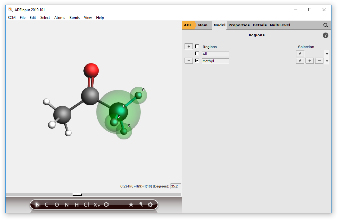
You have just defined a new region, with a name ‘Methyl’. In your molecule window you can see what atoms are part of this region: they are highlighted with semi-transparent spheres. Note that there are now (at least) two regions define: the region that you defined, and a region called ‘All’ that is always present. Obviously, the All region includes all atoms. If you created the acetone molecule via the search command, you may have a third region that was automatically made.

Now we will define yet another region: the rest of the molecule. One way to do this is just to select the atoms that should be part of it, and pressing the ‘+’ button as you did before. However, to demonstrate some of the things you can do with regions we will do it in another way:

Make sure you have only the All and the Methyl region; if you have more, press the ‘-‘ button in front of the region

Click the check button in the ‘All’ region

Click the ‘+’ button to create a new region, as you did before

Click the check button in the ‘Methyl’ region

Click the ‘-‘ button in the ‘Region_2’ line, on the right-hand side

Basically, what you just did: select all atoms, make a new region containing all atoms, select the atoms in the Methyl region, remove the selected atoms from the new region. By clicking on the select buttons in the regions you can easily verify that your regions are now as they should be.

Tip

Shortcut to quickly generate a new region containing the selection: Atoms → New Region From Selected Atoms, or cmd/ctrl - G.

Visualization options per region

You can easily change what regions, and atoms within that region look like:

Click in empty (drawing) space to clear the selection

Click in the check box in front of the ‘Methyl’ region name to uncheck it

You should observe that the ghost-like region visualization disappears. Please turn it back on:

Click in the check box in front of the ‘Methyl’ region name to check it

Click on the right arrow at the end of the ‘Region_2’ line

Use the ‘Sticks’ command from the menu that appears

Now anything in ‘Region_2’ will be visualized as sticks only. Obviously you could also select any of the other display options.

Using regions to group molecules for editing

You can use regions to group atoms together for editing. When changing the distance, angle or dihedral using the slider atoms that are in one region move together.

As an example, lets break the aceton molecule into three fragments by deleting the C-C bonds:

Delete the CC bonds

Note that one CH3 fragment and the CO group are still together in one region, and the other CH3 group is in its own region.

Select the C from the CO group and the C from the CH3 group that is in a different region

(use shift-click on an atom to add atoms to the selection)

Use the slider to change the distance between the selected carbons

Note that the CO group and the CH3 group in the same region move together, thus the regions act as a tool to group things together for editing (with the slider). This grouping also works when you want to change an angle using the slider.

To prepare for the next step of the tutorial, undo the changes you made in this step using the Undo function repeatedly:

Undo until the C-C bonds are present again

Step 2: QUILD

Once you have defined your regions, it is easy to set up the QUILD calculation:

Use the panel bar ADF → Quild menu to select the Quild panel

Click the ‘+’ button to add an action

Click the ‘+’ button to add a second action

In the first action, select DFTB in the ‘Use’ field

In the second action, select ADF in the ‘Use’ field

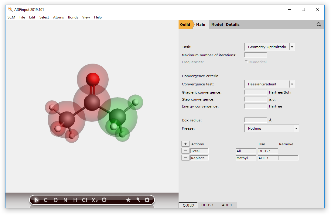
The first action (‘Total’) defines what to do with the full molecule. It normally will apply to the entire molecule, and thus the ‘All’ region is preselected. In the ‘Use’ field you have specified how to treat the whole molecule: with DFTB.

The second action (‘Replace’) tells QUILD to replace the DFTB result for the selected region with results from another method. The region for which we want to do this is the ‘Methyl’ region, and it happens to be automatically selected. You can use the region pull-down menu will to select another region, and it offers you a short-cut to make a new region.

In the ‘Use’ field of the second action you have selected what to use as a replacement method: ADF.

In the ‘Remove’ field it should be specified that you wish to remove the DFTB results for this region. ADFinput will enter this automatically when you save your job. You can also set it manually if you wish.

The Quild panel offers you to set some details for the QUILD calculation. The defaults should work fine.

Save your set up

Four tabs can be found at the bottom of the Quild panel: ‘Quild’, ‘DFTB 1’, ‘ADF 1’ and ‘DFTB 2’. These tabs allow you to set up the different parts of the calculation. Right now you could make adjustments of the global QUILD settings. If you press on the ‘ADF 1’ tab, you will have the option to set the details of the ADF calculation (for the ‘Methyl’ region). And if you click on the ‘DFTB 1’ tab you can set up details of the DFTB part of the calculation. The ‘DFTB 2’ tab is the DFTB calculation on the ‘Methyl’ group that will be removed from the full system. Normally the set up for this calculation is identical to the full system (DFTB 1), but in some special cases you will need to modify it. See the QUILD manual for details.

Click on the ‘ADF 1’ tab

Look through the different panels, to see what options ADF will use. Do NOT make changes!

Click on the ‘DFTB 1’ tab

Select the DFTB.org/3ob-3-1 parameter set

Click on the ‘DFTB 2’ tab

Select the DFTB.org/3ob-3-1 parameter set

Click on the ‘Quild’ tab

Save your set up

Now let’s run this calculation:

File → Run

Click ‘No’ when asked to update the geometry

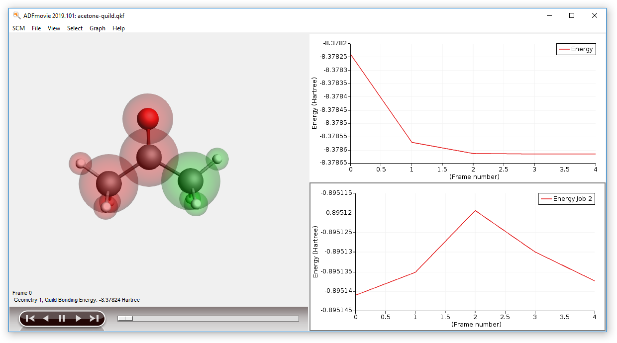
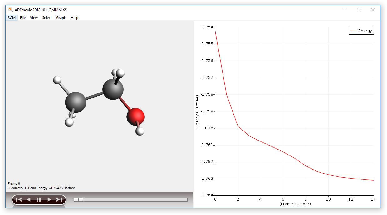
When your calculation is finished you can view the resulting optimization using ADFmovie:

Use the SCM → Movie command

Add a second graph: Graph → Add Graph

Show the energy of the ADF-subsystem on the second graph:

Graph → Quild Energies → job 2 : ADF ...

You can also open the output file using the SCM → Output command. The other visualization tools can not be applied to the full QUILD results, but they can be used to examine the result of the ADF calculation (on the Methyl region). This is done in quildjob.2:

Show the ADFjobs window

Show the QUILD job details (click on the triangle to show the details)

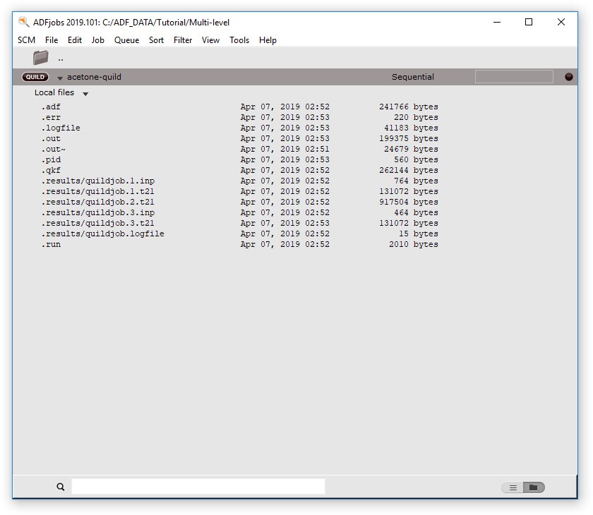
Using the View menu command you will try to open the .t21 result file for the QUILD job. That will not work, we need to view only the .t21 file of the adf sub-system. To do this, we first open this result file in the KFBrowser. This tool allows you to inspect details of the binary KF files. Next, use the View command in the SCM menu of the KFBrowser to open that specific file in ADFview:

Double-click on the .results/quildjob.2.t21 file

In the KFBrowser window, SCM → View

In the ADFview window Remove and Guess bonds (this is a work-around a bug that messes up the bond display)

Visualize the HOMO in ADFview

Click on the Isosurface: With Phase pull-down menu and use the Show Details command

Change the Opacity to 70

Note that QUILD has added a dummy hydrogen to cap the broken bond.

In the ADFview window, use the SCM → Levels command

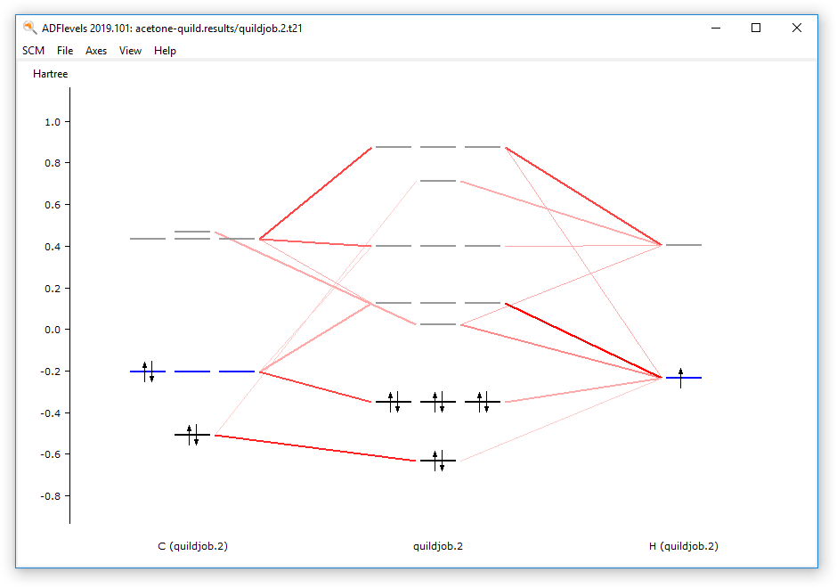
Now you have the ADF result file for the methyl group visible in ADFview and ADFlevels. With ADFview and ADFlevels you can examine the ADF results as usual.

SCM → Quit All

Step 3: QMMM

Generate ethanol in water

To demonstrate how to set up a QM/MM calculation using ADFinput, we will use ethanol in water as an example. This will also show you how to add explicit solvent molecules to your system:

Start ADFinput

Build an ethanol molecule

Pre-optimize the structure

Edit → Solvent Molecules...

Change the radius of the solvent sphere to a small value,

such that 10 solvent molecules will be generated

Click on ‘Add Solvent’

As you can see, ADFinput has generated 10 water molecules around your ethanol molecule. It also has created two regions: a Solute region containing the ethanol molecule, and a Solvent region containing the water molecules. The visualization option for the Solvent region is such that the water molecules will only be shown using a Wire-frame representation.

Set up the QM/MM calculation

The next step is to set up the QM/MM calculation:

ADF → QMMM: select the ‘QMMM’ panel

Select the ‘Solute’ region in the ‘QM Region’ pull-down menu

Change the QMMM Task to Geometry Optimization

Now you will have three tabs: the main QMMM tab that allows you to set QMMM details, the ‘ADF 1’ tab that is the setup for the ADF calculation for the Solute subsystem, and the ‘MM 5’ tab that sets up the MM calculation for the full system.

ADFinput is currently not very smart in setting the proper atom types for a MM calculation. So you will need to examine the atom types as they are generated in the MM input, and fix them if they are not correct. To fix this, if needed, use the Atom Inspector panel to set the Tripos (or Amber) atom types as needed.

Click on the ‘MM 5’ tab

Activate the ‘Run Script’ panel (in the panel bar Details)

Check the atom types (in the run script)

Run the QMMM calculation, and see results

Run your calculation File → Run

Show the optimization movie:

In the ADFinput window: SCM → Movie

Graph → Energy

Note that ADFmovie (and the other GUI modules) will only show the results for the QM part of your calculation.

To get detailed information on your QMMM calculation, you can check the output file using the SCM → Output command.

Step 4: DRF

Introduction

To demonstrate how to set up a DIM/QM DRF calculation using ADFinput, we will use water in water as an example. DRF is a QM/MM method in which the MM atoms interact with the QM region via induced dipoles and static charges. DRF facilitates calculating the optical properties of molecules, in this case we will look at the solvent effect on excitation energies. Note that the geometry optimizations are not possible with DRF in ADF.

Gas phase excitation energies

Start ADFinput

Build a water molecule

Pre-optimize the structure

Use the ADF panel

Select the Single Point task

Use the panel bar Properties → Excitations (UV/Vis), CD command

For the ‘Type of excitations’ option, Select ‘SingletOnly’

Save as ‘Water’

File → Run

Solvent effects excitation energies using DRF

Edit → Solvent Molecules...

Change the radius of the solvent sphere to a value,

such that approximately 130 solvent molecules will be generated

Click on ‘Add Solvent’

Use the panel bar Model → DIM/QM command

For the ‘Method’ option, Select ‘DRF’

Click the check button ‘QM part’ for the Solute region

Click the check button ‘DIM part’ for the Solvent region

In the next step atomic charges for the DRF region are computed using MDC-Q charges (LDA functional, DZP basis set). The atomic polarizabilities are taken from a inner database including H, C, N, O, F, S, Cl, Br, I atoms.

For the ‘Select charges’ option, Select ‘MDC-Q’

Save as ‘Water_DRF’

File → Run

See the results

When the calculation is ready, select both the Water_DRF and the Water job in ADFjobs

Open ADFspectra: SCM → Spectra command

Axes → Horizontal Unit → eV

Note that having two jobs selected in ADFjobs opens both jobs in the same ADFspectra window. That is easy to compare results.

Alternatively (with the same result), open ADFspectra for one of the jobs, and use the Add command in the File menu.

Step 5: Quality per region

Another method to handle bigger systems is to calculate part of your system as you would normally do, and another part that further away of the region of interest with a lower numerical accuracy, and/or smaller basis sets. As an example how to set this up we will use the same ethanol - water solvent system that was used for the QM/MM tutorial in the previous step.

Start ADFinput

Build an ethanol molecule

Pre-optimize the structure

Edit → Solvent Molecules...

Change the radius of the solvent sphere to a small value,

such that 10 solvent molecules will be generated

Click on ‘Add Solvent’

Note that your system consists of two regions: the Solute and the Solvent region.

The next step is to set up the calculation parameters:

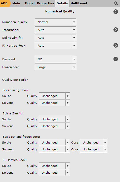
Select the Geometry Optimization task

Use the button on the “Numerical Quality” line

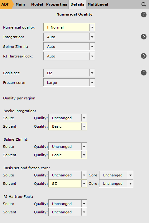
For the Solvent region:

change the Becke integration to Basic

change the Spline Zlm fit to Basic

change the Basis quality to SZ

Next run the calculation and see a movie of the results:

Run your calculation File → Run, save with a name you like

Show the optimization movie (while the job is still running):

In the ADFinput window: SCM → Movie

Note that now you will see the full system, in contrast with the QM/MM results. As the gradient convergence information is available from the logfile, ADFmovie will automatically show not only the Energy curve, but also the gradient convergence curves.

Depending on your exact starting geometry the optimization may need many cycles. As this is just a tutorial, there is no point in waiting for it. So you may just kill it:

In ADFjobs select your job

If it is still running: Job → Kill