PES scan, transition state search and IRC

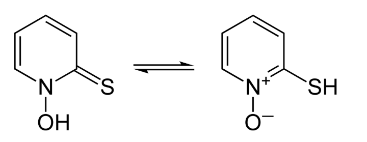
In this tutorial we will locate the transition state for Pyrithione tautomerization:

Specifically, we will use AMS in combination with the DFTB Engine to:

• Perform a 1D Potential Energy Surface (PES) scan, a.k.a. linear transit, to locate the initial guess for the subsequent Transition State (TS) search
• Compute the Hessian and normal modes by performing a Frequencies calculation
• Perform a transition state search using the Hessian computed in the previous step
• Compute the Intrinsic Reaction Coordinate (IRC) path connecting the reactant and the product

More informations on these features can be found in the AMS User manual:

• PES scan section of the AMS manual
• Properties section of the AMS manual
• Transition State search section of the AMS manual
• Intrinsic Reaction Coordinate section of the AMS manual

PES Scan

Let us begin by starting up the ADFInput GUI module:

1. Start ADFjobs

2. Click on SCM → New Input. This will open ADFInput

3. In ADFInput, select the DFTB panel: ADF → DFTB

To create the Pyrithione molecule:

Copy-paste the following coordinates in the Molecule Editing Area of ADFInput

13

C      -2.30800400      -0.33458354      -0.03944688
C      -3.55161726      -0.98161691      -0.01806157
C      -3.59405760      -2.37377447       0.06998894
N      -2.43475599      -3.05706858       0.13215278
C      -1.19114674      -2.47716286       0.11543345
C      -1.13146988      -1.07344958       0.02678424
H      -4.47776711      -0.41946857      -0.06866615
H      -4.51286388      -2.95462913       0.09224655
O      -2.42829502      -4.40191846       0.21755293
S       0.09533105      -3.63607352       0.21049529
H      -0.16385857      -0.58321314       0.01095504
H      -2.26672769       0.74932834      -0.10794508
H      -1.26310602      -4.50300286       0.24347732

We now need to select the task and the DFTB parameter set:

1. In the main panel, select Task → PES Scan

2. Click on the folder next to Parameter directory and select DFTB.org/3ob-3-1

Your ADFInput window should look like this:

Now switch to the “Geometry Constraints and PES Scan” input panel:

In the menu bar, select Model → Geometry Constraints and PES Scan

We will now set up the coordinate along which to scan the potential energy surface:

In the Pyrithione tautomerization, the hydrogen atom bonded to oxygen will cross a small energy barrier and bond to the sulfur atom next to it. We will therefore scan the energy as a function of the H-S distance:

1. Select the H atom attached to O

2. Holding down Shift, select the S atom

3. Click on + next to H(13) S(10) (distance)

This will add the H-S distance as a scan coordinate.

We now need to set the initial value, final value and number of intermediate steps for the H-S distance:

1. Set initial distance to 1.612

2. Set final distance to 1.4

3. Set the number of scan points for coordinate SC-1 to 8

We are now ready to run the calculation:

1. Click on File → Save As... and give it the name “PES_scan”

2. Click on File → Run . This will bring the ADFJobs window to the front

3. Wait for the calculation to finish...

After the calculation is completed, we can visualize the results:

In ADFJobs, select the job “PES_scan” then click on SCM → Movie

This will open the ADFMovie program and show the energy profile of the PES scan.

With ADFMovie into focus, use the the right and left arrow keys to go through the frames

As initial guess for the TS search, we pick the geometry corresponding to the highest energy in the PES scan, i.e. frame number 3.

1. In ADFMovie, using either arrow keys or the slider, select Frame number 3

2. Click on File → Update Geometry in Input

This will bring ADFInput to the front update the geometry of the Pyrithione molecule.

Frequencies calculation

It is important to have a good starting Hessian with one imaginary frequency when performing a TS search.

Here we calculate the Hessian matrix that will be used in the subsequent TS search.

In ADFInput:

1. In ADFInput, go to the Main panel

2. Select Task → Single Point

3. Select Followed by → Frequencies

We can now run the Frequency calculation, which will compute the Hessian and the normal modes:

1. Click on File → Save As... and give it the name “Frequencies”

2. Click on File → Run . This will bring the ADFJobs window to the front

3. Wait for the calculation to finish...

When the calculation is finished, we can visualize the normal modes using ADFSpectra:

In ADFJobs select the job “Frequencies” then click on SCM → Spectra

This will open ADFSpectra:

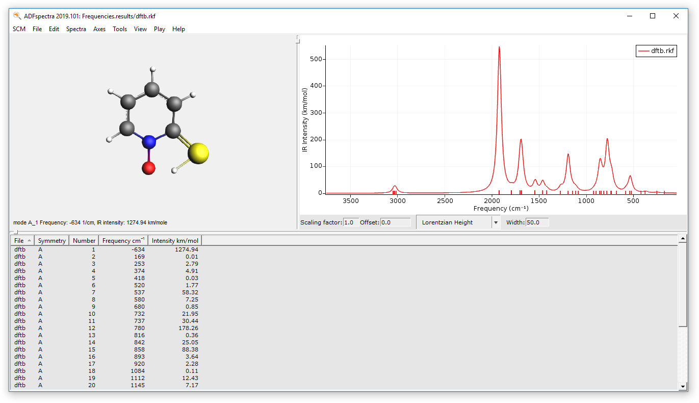
The first mode should have an imaginary frequency (which in the table is shown as a negative frequency). Click on the line in the table corresponding to the imaginary frequency to visualize the mode.

We are now ready to perform the TS search.

Transition state search

1. Open the ADFInput window of the job “Frequencies”

2. Select Task → Transition State

3. Make sure that Followed by is set to Frequencies

The main panel should look like this:

1. Go to the panel Details → Geometry Optimization

2. Select Initial Hessian → From File

3. click on the folder next to Initial Hessian From:

4. Select the file dftb.rkf in the folder Frequencies.results

Note that ADFInput still carries the geometry constraint from the previous PES scan calculation, which has to be removed before starting the new calculation:

1. Go to the panel Model → Geometry Constraints and PES Scan

2. Remove the H(13) S(10) constraint by clicking on - in front of it

We can now run the TS search calculation:

1. Click on File → Save As... and give it the name “TS”

2. Click on File → Run . This will bring the ADFJobs window to the front

3. Wait for the calculation to finish...

4. Click on Yes when ADFInput asks whether to “Read new coordinates from...”

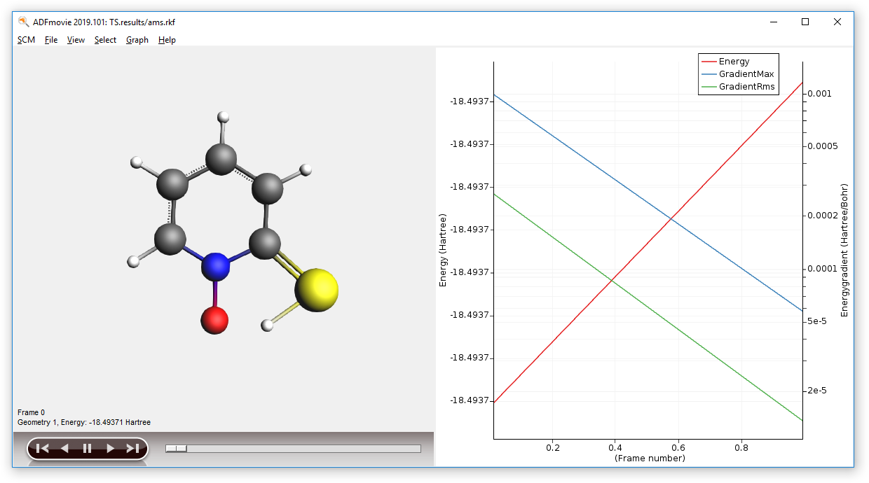
You can now visualize the TS search using ADFMovie:

In ADFJobs select the job TS and select SCM → Movie

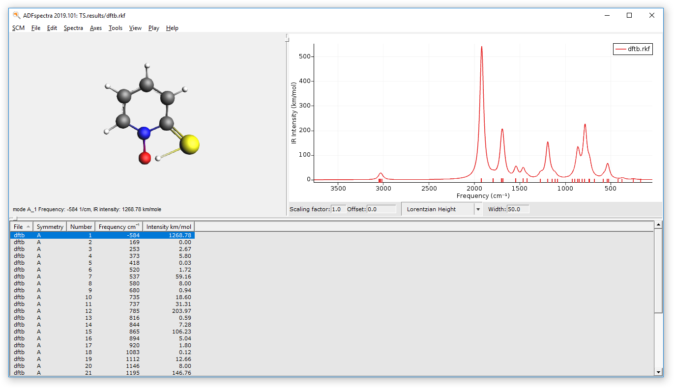
And confirm that the there is exactly one imaginary (negative) frequency by inspecting the IR spectra with ADFSpectra:

In ADFJobs select the job TS and select SCM → Spectra

IRC (Intrinsic Reaction Coordinate) calculation

1. Open the ADFInput window of the job “TS”

2. In the main panel select Task → IRC

3. Select Followed by → Nothing

4. Click on next to Task → IRC

In the IRC panel you can adjust the options for the Intrinsic Reaction Coordinate calculation. For this example the default options are fine.

We can now run the IRC search calculation:

1. Click on File → Save As... and give it the name “IRC”

2. Click on File → Run . This will bring the ADFJobs window to the front

3. Wait for the calculation to finish...

You can now visualize the IRC path using ADFMovie:

In ADFJobs select the job IRC, then select SCM → Movie

A summary of the IRC calculation can be found at the end of the output file:

1. In ADFJobs select the job IRC, then select SCM → Output

2. Scroll until the end of the output file to see the IRC summary:

 ---------------------------------------------------------------
                         IRC summary
System energy at the TS                  -18.49370493 Hartree
Forward barrier height                     0.00022713 Hartree
Backward barrier height                    0.00245861 Hartree
---------------------------------------------------------------
        Rel. energy   Rel. energy    Path coord   RMS gradient
          [Hartree]    [kcal/mol]    [Angstrom]    [Hartree/A]
    1    -0.0024586        -1.543      -0.47694      0.0000169
    2    -0.0024368        -1.529      -0.44378      0.0004731
    3    -0.0022943        -1.440      -0.39267      0.0013751
    4    -0.0020017        -1.256      -0.33119      0.0022516
    5    -0.0015350        -0.963      -0.26152      0.0030561
    6    -0.0008980        -0.563      -0.17942      0.0031652
    7    -0.0002510        -0.157      -0.10353      0.0025638
    8     0.0000000         0.000       0.00000      0.0000251 TS
    9    -0.0001465        -0.092       0.10315      0.0012826
   10    -0.0002271        -0.143       0.14237      0.0000498
---------------------------------------------------------------