TlH (thallium hydride) Spin-Orbit Coupling
This tutorial consists of several steps:
- TlH spin-orbit fragment analysis
- Separate calculations for Tl and H
- Visualization of the energy diagram
- Visualization of spinors
- Calculate the atomization energy
Step 1: Prepare molecule
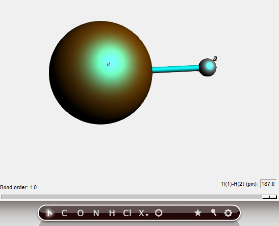
First create a TlH (thallium hydride) molecule with a bond length of 1.87 Angstrom (the experimental bond length):
- Open ADFinput and draw a TlH molecule.Select the Tl and H atomsUse the slider to set the distance between the atoms 1.87 Angstrom
Step 2: Set calculation options
Next we will set up the calculation. The following details need to be set:
- Clear the selection (click in empty drawing space)Select the GGA → BP86 as XC functionalSelect the ‘Spin-Orbit’ Relativity optionSelect the basis set ‘TZ2P’Set Frozen core to ‘None’
The Main panel will now look like:

We are going to perform a fragment analysis as a trick to get a diagram that makes it very easy to compare scalar and spin-orbit relativistic results.
Fragment calculations are based on regions, which are just collections of atoms. So we start by making a region:
- Select both atomsUse the panel bar Model → Regions commandClick the ‘+’ button to add a new regionChange the name of the new region (Region 1) to TlH_SR

You have now defined a region containing all atoms, with name TlH_SR.
- Use the panel bar Multilevel → Fragments menu commandClick the ‘Use fragments’ check box

Step 3: Run your calculation
- Use the File → Save menu commandEnter the name ‘TlH_SO’ in the ‘Filename’ fieldClick ‘Save’
Now you have saved your current options and molecule information.
As we have set up a fragment calculation, also the .adf and .run files for the fragment have been saved. Lets study what options are used for the fragment in ADFinput:
- Make sure the ‘Fragments’ panel is still the current panelClick on the ‘Open’ button (the dot) for the TlH_SR fragment
A new ADFinput window will also appear with the name ‘ADFinput: TlH_SO.TlH_SR.adf’. This is the name of the molecule, a dot, and the name of the fragment. The fragment should have the ‘Scalar’ relativistic option selected, as that is required when the results will be used as a fragment. The other options are identical to what you set for the main molecule.
Now close this ADFinput window:
- Select the ADFinput window with the name ‘ADFinput: TlH_SO.TlH_SR.adf’Select File → Close
We are now ready to run the calculation:
- Select the ADFinput window with the name ‘TlH_SO.adf.Select File → Run
Now two calculations will run: first the building fragment (using the scalar relativistic option), and next the version including spin-orbit coupling. You will see the two logfiles. Wait until both calculations have finished:
- Wait until ADFtail shows ‘Job ... has finished’ as last lineSelect File → CloseRepeat for the second ADFtail, thus closing both logfiles
Step 4: Results of the calculation
TlH energy diagram
To see the effect of the spin-orbit coupling we will first look at the energy level diagram:
- Select the ADFinput window with the name ‘TlH_SO.adf.SCM → LevelsSelect View → Labels → ShowPress and hold the Right mouse button on the stack name ‘TlH_SO’,Click on ‘Zoom HOMO-9 .. LUMO+9’.Next try to zoom using a drag with the right mouse button, or using the scroll wheel.Do this such that only levels between -0.1 and -0.7 eV are shown.You can move the levels vertically by dragging with the left mouse button.

You can see that the spin-orbit coupling is important to split energy levels.
Especially for the Tl core levels the spin-orbit coupling is more important than the ligand field splitting. Compare the 8pi, 13sigma, 4delta orbitals (close to 5d atomic Tl orbitals) with the 11j3/2, 20j1/2 spinors (close to 5d3/2 atomic Tl spinors) and 5j5/2, 12j3/2, and 21j1/2 spinors (close to 5d5/2 atomic Tl spinors).
If you press and hold the right mouse button on one of the levels, you can select a spinor. That spinor will be shown. You can also show all spinors (in the case of a degenerate level) at once.
The energy diagram of the scalar relativistic fragment calculation shows the atomic contributions to the scalar relativistic levels.
- Bring ADFjobs to the frontSelect the TlH_SO.TlH_SR job (the scalar relativistic fragment)Use the SCM → levels commandSelect View → Labels → ShowPress and hold the Right mouse button on the stack name ‘TlH_SO.TlH_SR’,Click on ‘Zoom HOMO-4 .. LUMO+4’.Next zoom and move the levels using a right mouse drag and or scroll wheel.

Visualization of spinors
Visualization of spinors is conceptually more difficult than visualization of orbitals.
A spinor \(\Psi\) is a two-component complex wave function, which can be described with four real functions \(\phi\): real part \(\alpha\) \(\phi_\alpha^R\) , imaginary part \(\alpha\) \(\phi_\alpha^I\) , real part \(\beta\) \(\phi_\beta^R\) , imaginary part \(\beta\) \(\phi_\beta^I\):
The density \(\rho\) is:
The spin magnetization density \(m\) is:
where \(\sigma\) is the vector of the Pauli spin matrices \(\sigma_x\), \(\sigma_y\), and \(\sigma_z\). A spinor is fully determined by the spin magnetization density and a phase factor \(e^{i \theta}\), which both are functions of spatial coordinates.
In ADFview one can visualize the (square root of the) density and spin magnetization density, however, the phase factor \(e^{i \theta}\) is summarized only with a plus or minus sign.
For this tutorial we have a small molecule, and a fine grid is chosen for better visualization.
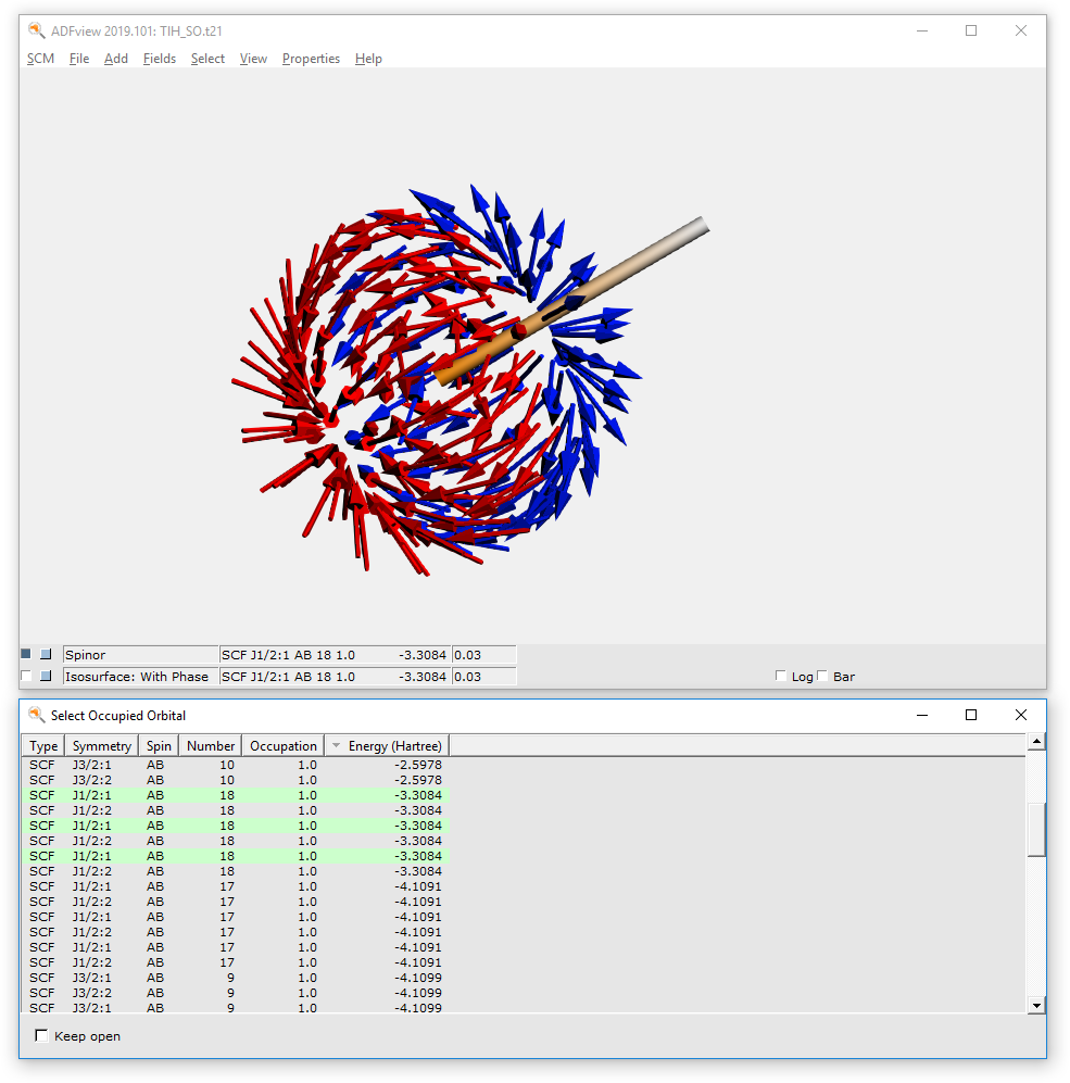
- Select the ADFinput window with the name ‘TlH_SO.adf.Select SCM → ViewRotate the molecule, such that one can see both atoms.Select Fields → Grid → FineSelect Add → Spinor: Spin Magnetization DensityIn the new control line at the bottom, use the field select pull-down menu andSelect Orbitals (occupied) ....Select the J1/2:1 number 22 spinor.

The arrows in this picture are in the direction of the spin magnetization density m. All arrows are approximately in the same direction, which means that this spinor is an eigenfunction of spin in this direction of the arrows. In fact this 22 j1/2 spinor is almost a pure \(\alpha\) orbital. The arrows are drawn starting from points in space where the square root of the density is 0.03. The color of the arrows is red or blue by default, indicating minus or plus for the phase factor \(e^{i \theta}\) .
The (square root of the) density and the approximate phase vector \(e^{i \theta}\) can also be viewed separately:
- Select Add → ‘Isosurface: With PhaseSelect Orbitals (occupied)...Select the SCF_J1/2:1 number 18 spinor.Hide the spinor (uncheck the check box at the left of the Spinor label)

This spinor 18j1/2 is almost a pure 5p1/2 Tl spinor. A p1/2 atomic orbital has a spherical atomic density, but a spin magnetization density which is not the same in each point in space.
- In the control line with ‘Spinor’, press on the pull-down menu andSelect Orbitals (occupied)Select the SCF_J1/2:1 number 18 spinorShow the ‘Spinor’ (check the left check box for the spinor line)Hide the ‘isosurface with phase’ (uncheck the left check box for the isosurface with phase line)Hide the atoms: View → Molecule → Sticks
Step 5: Calculate the atomization energy including spin-orbit coupling
The calculation of the atomization energy is not a simple problem in DFT. Spin-orbit coupling is an extra complication. In this paragraph a way is presented how to calculate the atomization energy using spin-polarized calculations in the non-collinear approximation.
If you wish, you can skip the rest of this tutorial.
The Tl atom
To calculate an atomization energy we need to calculate the atoms also including spin-orbit coupling. The easiest way is to start with the TlH_SO.adf file and change this to an atomic file.
Since the Tl atom is an open shell atom for an (accurate) atomization energy we need to do an unrestricted calculation. The best theoretical method is the non-collinear method. Note that the ‘Spin polarization’ field is not used in the non-collinear method.
- Select the ADFinput window with the name ‘TlH_SO.adfDelete the H atom (select it and press the backspace key)Use the panel bar Multilevel → Fragments commandUncheck the ‘Use fragments’ optionUse the panel bar Model → Regions commandRemove the TlH_SR region (click on the - button in front of it)Select ‘Main’ panelCheck the ‘Unrestricted:’ boxSelect the Relativity panel (search for relativity)Select ‘NonCollinear’ from the ‘Spin polarization’ optionsSelect File → Save AsEnter the name ‘Tl_SO’ in the ‘FileName’ fieldClick on ‘Save’Click OK to acknowledge the warning about fractional occupation numbers

Now we want to actually perform the calculation for the Tl atom
- Run the calculation: File → RunWait until ADFtail shows ‘Job ... has finished’ as last lineIn the window showing the logfile (the ADFtail window Tl_SO.logfile):Select File → Close
The H atom
Basically we can follow the same steps as for the Tl atom, but in this case we will start with Tl_SO.adf file and change this.
- Select the ADFinput window with the name ‘Tl_SO.adfSelect the ‘Main’ panelSelect the Tl atomUse the Atoms → Change Atom Type → HSelect File → Save As...Enter the name ‘H_SO’ in the ‘Filename’ fieldClick on ‘Save’Select File → RunWait until ADFtail shows ‘Job ... has finished’ as last lineIn the window showing the logfile (the ADFtail window H_SO.logfile):Select File → Close
TlH atomization energy
The atomization energy including spin-orbit coupling is a combination of several terms.
- Select the ADFinput window with the name ‘TlH_SO.adf.Select SCM → LogfileWrite down the value of the bonding energy printed at the end of the calculationin the ADFtail window. (should be around -1038.62 eV)Select File → OpenSelect the file ‘TlH_SO.TlH_SR.logfile’Write down the value of the bonding energy printed at the end of the calculationin the ADFtail window. (should be around -3.84 eV)Select File → OpenSelect the file ‘Tl_SO.logfile’Write down the value of the bonding energy printed at the end of the calculationin the ADFtail window. (should be around -1039.32 eV)Select File → OpenSelect the file ‘H_SO.logfile’Write down the value of the bonding energy printed at the end of the calculationin the ADFtail window. (should be around -0.95 eV)
The atomization energy including spin-orbit coupling is in this case, the bond energy printed in the TlH_SO.logfile plus the the bond energy printed in the TlH_SO.TlH_SR.logfile minus the bond energy printed in the Tl_SO.logfile minus the the bond energy printed in the H_SO.logfile. (approximately -1038.62 - 3.84 + 1039.32 + 0.95 = -2.19 eV, experimental number is close to -2.06 eV.)