Conformers Generation with Multiple Molecules¶

Worked Example¶

Lets see how two alanine molecules orient themselves using CREST conformer generation. To do this we will constrain the system in a spherical region using the SphericalWall constraint. We start by setting up a system of two alanine molecules in a relatively small space.

Initial imports¶

import scm.plams as plams
import sys
from scm.conformers import ConformersJob
import numpy as np
import matplotlib.pyplot as plt
import os

try:
    from scm.plams import view  # view molecule using AMSview in a Jupyter Notebook in AMS2026+

    _has_view = True
except ImportError:
    from scm.plams import plot_molecule  # plot molecule in a Jupyter Notebook in AMS2023+

    _has_view = False

    def view(molecule, ax=None, **kwargs):
        plot_molecule(molecule, ax=ax)


# this line is not required in AMS2025+
plams.init();

PLAMS working folder: /path/plams/examples/ConformersMultipleMolecules/plams_workdir

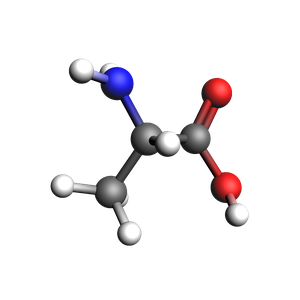
Single alanine molecule¶

smiles = "CC(N)C(=O)O"
alanine = plams.from_smiles(smiles)
view(alanine, height=300, width=300)

Initial system: alanine dimer¶

Pack two alanine molecules in a sphere with a density of 0.5 kg/L.

density = 0.5
mol = plams.packmol(alanine, n_molecules=2, density=density, sphere=True)

Translate the molecule to be centered around the origin (needed for SphericalWall later):

mol.translate(-np.array(mol.get_center_of_mass()))

view(mol, direction="along_pca3")

Calculation setup¶

To determine the radius of the SphericalWall we measure the size of the initial dimer.

dists = plams.distance_array(mol, mol)
max_dist = np.max(dists)
diameter = 1.33 * max_dist
radius = diameter / 2
print(f"Largest distance between atoms: {max_dist:.3f} ang.")
print(f"Radius: {radius:.3f} ang.")

Largest distance between atoms: 8.361 ang.
Radius: 5.560 ang.

Now we can set up the Crest conformer generation job, with the appropriate spherical wall constraining the molecules close together.

settings = plams.Settings()
settings.input.ams.EngineAddons.WallPotential.Enabled = "Yes"
settings.input.ams.EngineAddons.WallPotential.Radius = radius
settings.input.ams.Generator.Method = "CREST"
settings.input.ams.Output.KeepWorkDir = "Yes"
settings.input.ams.GeometryOptimization.MaxConvergenceTime = "High"
settings.input.ams.Generator.CREST.NCycles = 3  # at most 3 CREST cycles for this demo
settings.input.GFNFF = plams.Settings()

Run the conformers job¶

Now we can run the conformer generation job.

job = ConformersJob(molecule=mol, settings=settings)
job.run()
# ConformersJob.load_external("plams_workdir/conformers/conformers.rkf")  # load from disk instead of running the job

[12.01|12:36:00] JOB conformers STARTED
[12.01|12:36:00] JOB conformers RUNNING
[12.01|12:41:35] JOB conformers FINISHED
[12.01|12:41:35] JOB conformers SUCCESSFUL

<scm.conformers.plams.interface.ConformersResults at 0x1731ef880>

rkf = job.results.rkfpath()
print(f"Conformers stored in {rkf}")

Conformers stored in /path/plams/examples/ConformersMultipleMolecules/plams_workdir/conformers/conformers.rkf

This job will run for approximately 15 minutes.

Results¶

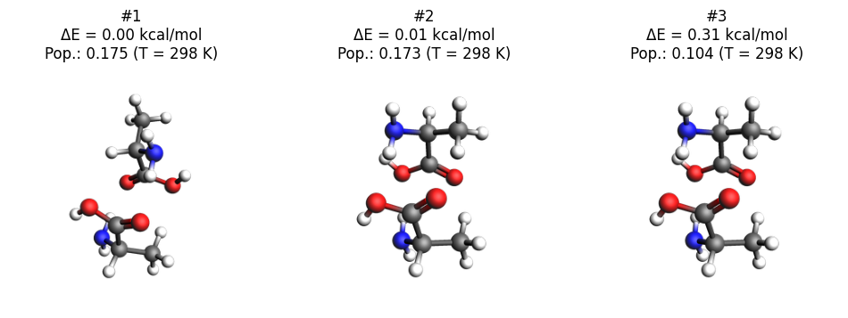
Here we plot the three lowest-energy conformers.

def plot_conformers(job: ConformersJob, indices=None, temperature=298, unit="kcal/mol", lowest=True):
    molecules = job.results.get_conformers()
    energies = job.results.get_relative_energies(unit)
    populations = job.results.get_boltzmann_distribution(temperature)

    if isinstance(indices, int):
        N_plot = min(indices, len(energies))
        if lowest:
            indices = list(range(N_plot))
        else:
            indices = np.linspace(0, len(energies) - 1, N_plot, dtype=np.int32)
    if indices is None:
        indices = list(range(min(3, len(energies))))

    fig, axes = plt.subplots(1, len(indices), figsize=(12, 4))
    if len(indices) == 1:
        axes = [axes]

    for ax, i in zip(axes, indices):
        mol = molecules[i]
        E = energies[i]
        population = populations[i]

        if _has_view:
            img = view(mol, width=300, height=300)
            ax.imshow(img)
            ax.axis("off")
            ax.set_title(f"#{i+1}\nΔE = {E:.2f} kcal/mol\nPop.: {population:.3f} (T = {temperature} K)")
        else:
            view(mol, ax=ax)
            ax.set_title(f"#{i+1}\nΔE = {E:.2f} kcal/mol\nPop.: {population:.3f} (T = {temperature} K)")

plot_conformers(job)

You can also open the conformers in AMSmovie to browse all conformers 1000+ conformers:

!amsmovie {rkf}

Finally in AMS2025+, you can also inspect the conformer data using the JobAnalysis tool.

try:
    from scm.plams import JobAnalysis

    ja = (
        JobAnalysis(standard_fields=None)
        .add_job(job)
        .add_field(
            "Id",
            lambda j: list(range(1, len(j.results.get_conformers()) + 1)),
            display_name="Conformer Id",
            expansion_depth=1,
        )
        .add_field(
            "Energies",
            lambda j: j.results.get_relative_energies("kcal/mol"),
            display_name="E",
            expansion_depth=1,
            fmt=".2f",
        )
        .add_field(
            "Populations",
            lambda j: j.results.get_boltzmann_distribution(298),
            display_name="P",
            expansion_depth=1,
            fmt=".3f",
        )
    )

    # Pretty-print if running in a notebook
    if "ipykernel" in sys.modules:
        ja.display_table(max_rows=20)
    else:
        print(ja.to_table())

except ImportError:
    pass

Conformer Id	E	P
1	0.00	0.175
2	0.01	0.173
3	0.31	0.104
4	0.33	0.100
5	0.59	0.065
6	0.87	0.040
7	0.89	0.039
8	1.10	0.028
9	1.14	0.026
10	1.36	0.018
…	…	…
1062	256.89	0.000
1063	306.67	0.000
1064	326.40	0.000
1065	369.67	0.000
1066	371.07	0.000
1067	415.00	0.000
1068	415.08	0.000
1069	470.42	0.000
1070	502.31	0.000
1071	666.28	0.000

Complete Python code¶

#!/usr/bin/env amspython
# coding: utf-8

# Lets see how two alanine molecules orient themselves using CREST conformer generation.
# To do this we will constrain the system in a spherical region using the `SphericalWall` constraint.
# We start by setting up a system of two alanine molecules in a relatively small space.

# ## Initial imports

import scm.plams as plams
import sys
from scm.conformers import ConformersJob
import numpy as np
import matplotlib.pyplot as plt
import os

try:
    from scm.plams import view  # view molecule using AMSview in a Jupyter Notebook in AMS2026+

    _has_view = True
except ImportError:
    from scm.plams import plot_molecule  # plot molecule in a Jupyter Notebook in AMS2023+

    _has_view = False

    def view(molecule, ax=None, **kwargs):
        plot_molecule(molecule, ax=ax)


# this line is not required in AMS2025+
plams.init()


# ## Single alanine molecule

smiles = "CC(N)C(=O)O"
alanine = plams.from_smiles(smiles)
view(alanine, height=300, width=300)


# ## Initial system: alanine dimer

# Pack two alanine molecules in a sphere with a density of 0.5 kg/L.

density = 0.5
mol = plams.packmol(alanine, n_molecules=2, density=density, sphere=True)


# Translate the molecule to be centered around the origin (needed for SphericalWall later):

mol.translate(-np.array(mol.get_center_of_mass()))


view(mol, direction="along_pca3")


# ## Calculation setup

# To determine the radius of the `SphericalWall` we measure the size of the initial dimer.

dists = plams.distance_array(mol, mol)
max_dist = np.max(dists)
diameter = 1.33 * max_dist
radius = diameter / 2
print(f"Largest distance between atoms: {max_dist:.3f} ang.")
print(f"Radius: {radius:.3f} ang.")


# Now we can set up the Crest conformer generation job, with the appropriate spherical wall constraining the molecules close together.

settings = plams.Settings()
settings.input.ams.EngineAddons.WallPotential.Enabled = "Yes"
settings.input.ams.EngineAddons.WallPotential.Radius = radius
settings.input.ams.Generator.Method = "CREST"
settings.input.ams.Output.KeepWorkDir = "Yes"
settings.input.ams.GeometryOptimization.MaxConvergenceTime = "High"
settings.input.ams.Generator.CREST.NCycles = 3  # at most 3 CREST cycles for this demo
settings.input.GFNFF = plams.Settings()


# ## Run the conformers job

# Now we can run the conformer generation job.

job = ConformersJob(molecule=mol, settings=settings)
job.run()
# ConformersJob.load_external("plams_workdir/conformers/conformers.rkf")  # load from disk instead of running the job


rkf = job.results.rkfpath()
print(f"Conformers stored in {rkf}")


# This job will run for approximately 15 minutes.

# ## Results
# Here we plot the three lowest-energy conformers.


def plot_conformers(job: ConformersJob, indices=None, temperature=298, unit="kcal/mol", lowest=True):
    molecules = job.results.get_conformers()
    energies = job.results.get_relative_energies(unit)
    populations = job.results.get_boltzmann_distribution(temperature)

    if isinstance(indices, int):
        N_plot = min(indices, len(energies))
        if lowest:
            indices = list(range(N_plot))
        else:
            indices = np.linspace(0, len(energies) - 1, N_plot, dtype=np.int32)
    if indices is None:
        indices = list(range(min(3, len(energies))))

    fig, axes = plt.subplots(1, len(indices), figsize=(12, 4))
    if len(indices) == 1:
        axes = [axes]

    for ax, i in zip(axes, indices):
        mol = molecules[i]
        E = energies[i]
        population = populations[i]

        if _has_view:
            img = view(mol, width=300, height=300)
            ax.imshow(img)
            ax.axis("off")
            ax.set_title(f"#{i+1}\nΔE = {E:.2f} kcal/mol\nPop.: {population:.3f} (T = {temperature} K)")
        else:
            view(mol, ax=ax)
            ax.set_title(f"#{i+1}\nΔE = {E:.2f} kcal/mol\nPop.: {population:.3f} (T = {temperature} K)")


plot_conformers(job)


# You can also open the conformers in AMSmovie to browse all conformers 1000+ conformers:


# Finally in AMS2025+, you can also inspect the conformer data using the JobAnalysis tool.

try:
    from scm.plams import JobAnalysis

    ja = (
        JobAnalysis(standard_fields=None)
        .add_job(job)
        .add_field(
            "Id",
            lambda j: list(range(1, len(j.results.get_conformers()) + 1)),
            display_name="Conformer Id",
            expansion_depth=1,
        )
        .add_field(
            "Energies",
            lambda j: j.results.get_relative_energies("kcal/mol"),
            display_name="E",
            expansion_depth=1,
            fmt=".2f",
        )
        .add_field(
            "Populations",
            lambda j: j.results.get_boltzmann_distribution(298),
            display_name="P",
            expansion_depth=1,
            fmt=".3f",
        )
    )

    # Pretty-print if running in a notebook
    if "ipykernel" in sys.modules:
        ja.display_table(max_rows=20)
    else:
        print(ja.to_table())

except ImportError:
    pass