Quantum ESPRESSO: Calculating IR and Raman Spectra¶

Computational Methodology¶

The calculation of IR and Raman spectra using Quantum Espresso (QE) involves a series of steps that are handled internally by AMS, making the process transparent to the user. These steps use the QE tools pw.x, ph.x, and dynmat.x. For detailed information about these tools, refer to the official Quantum Espresso documentation online.

Starting from an optimized geometry, a self-consistent field (SCF) calculation is performed using pw.x to determine the electronic ground state of the system. This step solves the Kohn-Sham equations iteratively to obtain the converged electron density and ground state energy. Next, ph.x is employed to calculate the phonon frequencies and eigenvectors at a specific q-point (typically \(\Gamma\) point) in the Brillouin zone using density functional perturbation theory (DFPT) to compute the dynamical matrix, which captures the interatomic force constants. Finally, dynmat.x is used to post-process the phonon data, obtaining the IR and Raman intensities, frequencies, and vibrational modes. This step involves computing the Born effective charges and the Raman tensors, which describe the coupling of the vibrational modes to the electric field and the change in polarizability, respectively. These quantities are essential for determining the IR and Raman activity of the vibrational modes.

IR and Raman spectra can be calculated using Quantum Espresso through AMS via two main interfaces: the graphical user interface (GUI) and the Python library, PLAMS. The GUI presents a user-friendly, visual approach that is ideal for users performing routine calculations on simple systems. It simplifies the process of setting up input files and visualizing results. On the other hand, PLAMS offers a powerful and flexible Python environment suitable for complex workflows, parameter sweeps, and integration with other scientific libraries. This makes it particularly advantageous for advanced users, high-throughput calculations, or situations that require automation and scripting, providing greater control and customization of the computational process. In this tutorial, we will explore both options. They are completely independent, so you can jump directly to the section that interests you the most.

Using the GUI¶

We will use the following structure as basis for the subsequent calculations:

Be       0.0000000000       1.5555413800       0.0007009000
Be       1.3471383600       0.7777706900       2.1887103500
 O       0.0000000000       1.5555413800       1.6512462200
 O       1.3471383600       0.7777706900       3.8392556700
VEC1    2.6942767100     0.0000000000     0.0000000000
VEC2   -1.3471383600     2.3333120800     0.0000000000
VEC3    0.0000000000     0.0000000000     4.3760188900

Setting Up the Calculation:

1. Open AMSinput

2. Copy & paste the coordinates above into AMSinput.

3. Switch to

4. Select Task → GeometryOptimization

5. Change the Wavefunction energy cutoff to 25 Ryd

6. Change the K-Points N to 4 4 3

You should get something like this:

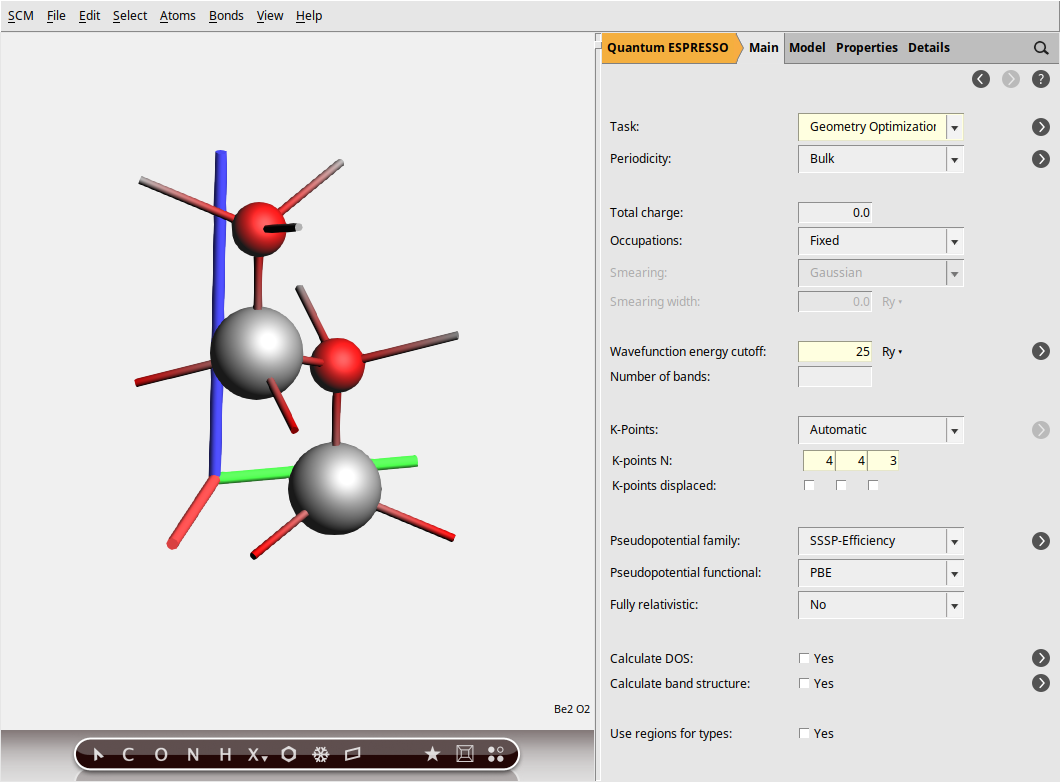
In the steps above, we specified a GeometryOptimization task to ensure our BeO structure is at a local energy minimum, preventing any spurious imaginary frequencies in the phonon spectrum. Next, for the electronic structure part, we set the plane-wave energy cutoff (ecutwfc) to 25 Ry. While this value is lower than typically recommended for production calculations (40 Ry), we use it here for demonstration purposes to reduce computational cost. Then, the Brillouin zone sampling is done using a Monkhorst-Pack k-point grid of size 4 × 4 × 3, ensuring a balanced sampling in all directions.

To specify the pseudopotentials, go to the Pseudopotentials configuration panel by selecting Model → Pseudopotentials. In this panel, use the file selection areas next to each element under “Pseudopotentials used:”. Clicking on the folder icon will open a file browser window. Navigate to the “QE” directory and select the appropriate pseudopotential file for each element.

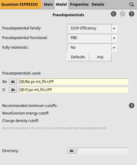
Notice that we have specified the pseudopotentials by selecting the files directly instead of using a pseudopotential family. This is due to Quantum Espresso’s limitation of only supporting Norm-Conserving (NC) and LDA-type pseudopotentials for Raman spectra calculations, which are not included in our standard pseudopotential families. For this example, we selected the pseudopotential files: Be.pz-mt_fhi.UPF for beryllium and O.pz-mt_fhi.UPF for oxygen. The filenames of these pseudopotentials indicate that they use the Perdew-Zunger LDA functional (pz), the Martins-Troullier generation method (mt), and that they originate from the FHI-aims library (fhi).

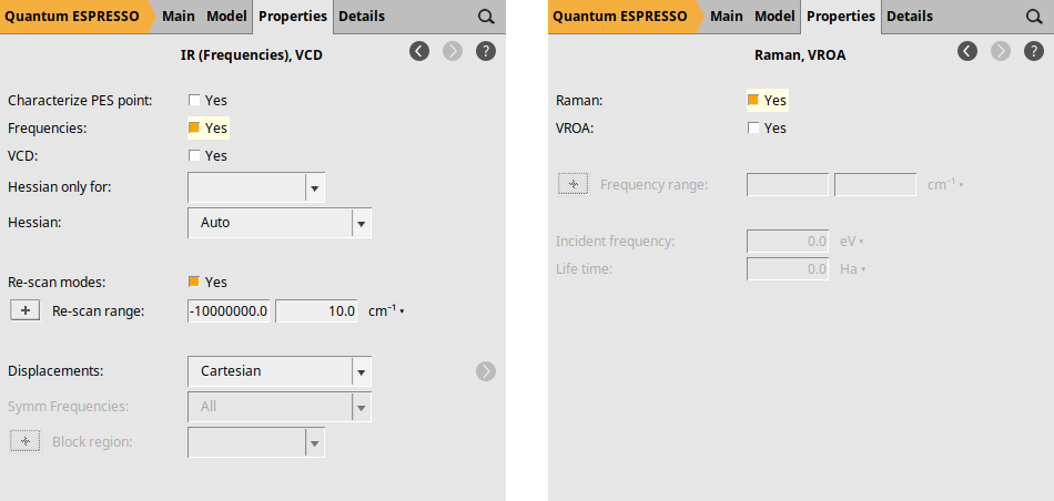
Finally, we explicitly request the calculation of NormalModes (which yields the IR spectrum) and the Raman spectrum. To request the IR spectrum, go to Properties → IR (Frequencies), VCD and check the box next to Frequencies: by selecting Yes. For the Raman spectrum, navigate to Properties → Raman, VROA and select Yes in the Raman: checkbox.

Computation & Results¶

We are now ready to start the calculation

1. Select File → Save As and give it an appropriate name (e.g. BeO)

2. Select File → Run

3. Wait for the calculation to finish (this should take a few minutes). Click Yes when asked to load the optimized geometry in AMSinput.

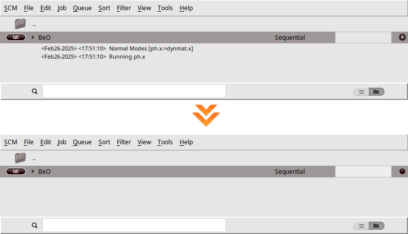
When you run a calculation, AMSjobs should come to the forefront, and your job will appear at the top of the list. On the right side, you’ll see the job running, indicated by a gear icon. While the simulation is in progress, the AMSjobs window will display the progress based on the logfile. Once the job is complete, the job status icon will change to a full circle to indicate that it is ready.

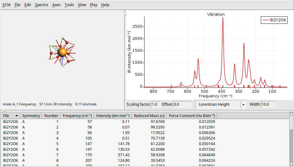
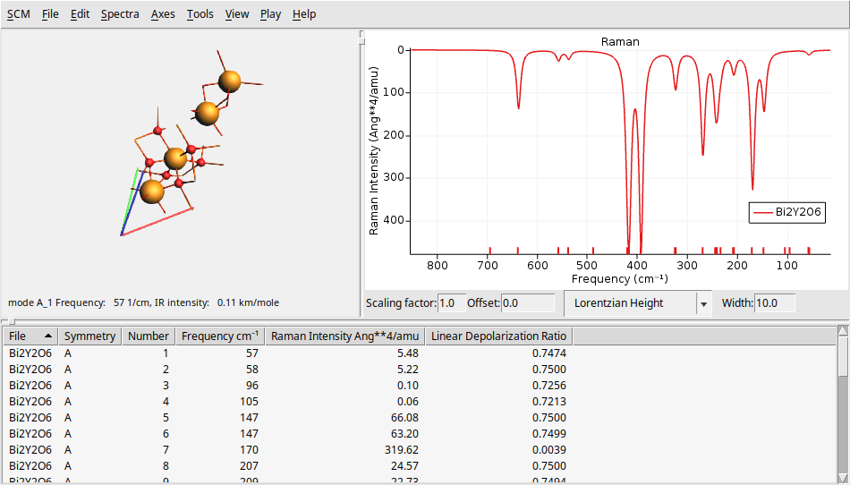
The AMSspectra module allows you to analyze both the IR and Raman spectra:

In AMSjobs (with your job selected) or AMSinput

Start the AMSspectra module by clicking (SCM → Spectra)

You should get something like this:

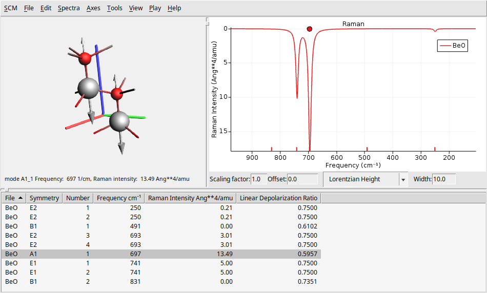
On the left side, there is a 3D representation of the BeO molecule, displaying the movement of atoms according to the selected normal mode. The right panel presents the calculated Raman spectrum. At the bottom, you will find a table that provides detailed information about each vibrational mode, including its symmetry, frequency, and Raman intensity.

Note

You can click on a vibrational mode in the bottom table or the Raman spectrum to see the atoms moving according to that mode’s vibrational frequency.

Note

To view the overlay arrows that indicate the displacement vectors for a specific vibrational mode, click on Play → Displacement Vectors. You can adjust the size of these arrows by using Ctrl + L to make them larger or Ctrl + K to make them smaller. Note that the figure above uses larger arrows than the default size.

Note

You can change several parameters related to the spectrum and its broadening using the text boxes at the bottom of the spectrum. You can modify the scaling factor and offset (useful for DFT functional correction factors), as well as the shape (such as Gaussian or Lorentzian) and the width. Note that the figure above uses a width of \(10.0\text{cm}^{-1}\), which may differ from your default value.

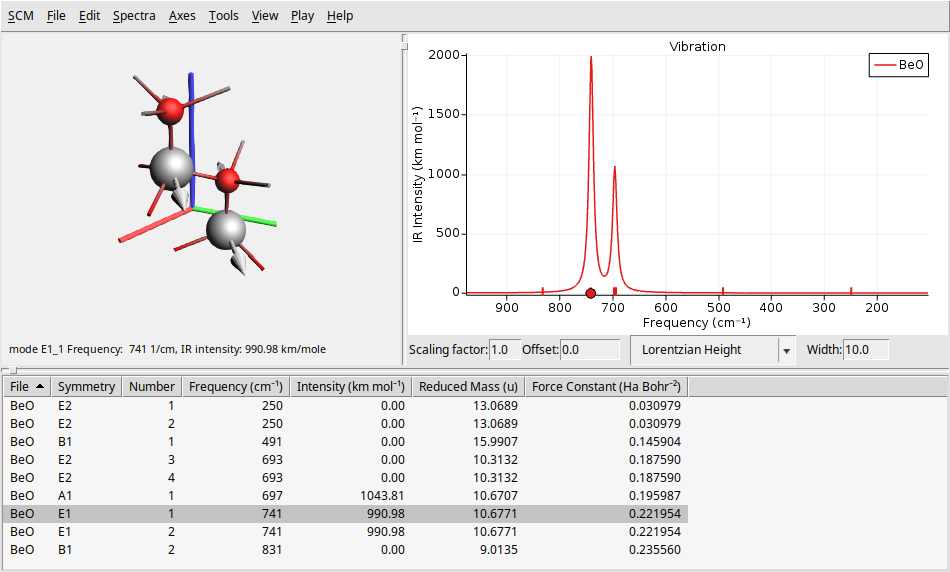
To see the IR spectrum go to Spectra → Vibration. This will refresh the window to display the IR spectrum results in a layout similar to that of the Raman spectrum.

As we said before, our system BeO has a hexagonal structure with symmetry \(C_{6v}\) (6mm) symmetry. So, we can verify if the transitions found in our calculations are in agreement with the table of characters of the point group \(C_{6v}\)

Table 15 Character table for point group \(C_{6v}\)¶

\(C_{6v}\)	E	\(2C_6(z)\)	\(2C_3(z)\)	\(C_2(z)\)	\(3σ_v\)	\(3σ_d\)	lin, rot	quadrat
\(A_1\)	+1	+1	+1	+1	+1	+1	\(z\)	\(x^2+y^2, z^2\)
\(A_2\)	+1	+1	+1	+1	-1	-1	\(R_z\)	–
\(B_1\)	+1	-1	+1	-1	+1	-1	–	–
\(B_2\)	+1	-1	+1	-1	-1	+1	–	–
\(E_1\)	+2	+1	-1	-2	0	0	\((x, y) (R_x, R_y)\)	\((xz, yz)\)
\(E_2\)	+2	-1	-1	+2	0	0	–	\((x^2-y^2, xy)\)

Note

Infrared selection rules:

If a vibration results in a change in the dipole moment, it is IR-active. These vibrational modes have the same symmetry as the \(x\), \(y\), and \(z\) axes.

Raman selection rules:

If a vibration results in a change in the polarizability, it is Raman-active. These vibrational modes have the same symmetry as quadratic functions like \(xy\), \(xz\), and \(x^2-y^2\).

From the characters table above, we can anticipate the IR and Raman activity of the BeO vibrational modes. This table indicates that modes with \(A_1\) and \(E_1\) symmetry should be IR-active, while modes with \(A_1\), \(E_1\), and \(E_2\) symmetry should be Raman-active. Notice this analysis is consistent with the results obtained from our calculations, as shown in the IR and Raman spectra plots above (see the columns symmetry and intensity at the bottom table).

Using Python (PLAMS)¶

To start, we import the matplotlib library, which is essential for visualizing different aspects of our calculations, such as molecular geometry, as well as the resulting IR and Raman spectra. By setting plt.rcParams['figure.dpi'] = 120, we adjust the resolution of the figures to ensure they are displayed with sufficient clarity and detail.

import matplotlib.pyplot as plt
plt.rcParams['figure.dpi'] = 120

As previously mentioned, we use the PLAMS Python library to interact with AMS. The code below constructs the beryllium oxide (BeO) crystal structure by defining a Molecule object. Individual atoms, beryllium (Be) and oxygen (O), are then added to the molecule using their respective symbols and Cartesian coordinates, which are specified in Angstroms. Next, the crystal lattice is defined as a 3x3 matrix, with dimensions also in Angstroms.

from scm.plams import Molecule, Atom

mol = Molecule()
mol.add_atom(Atom(symbol="Be", coords=(0.00000000, 1.55554138, 0.00070090)))
mol.add_atom(Atom(symbol="Be", coords=(1.34713836, 0.77777069, 2.18871035)))
mol.add_atom(Atom(symbol= "O", coords=(0.00000000, 1.55554138, 1.65124622)))
mol.add_atom(Atom(symbol= "O", coords=(1.34713836, 0.77777069, 3.83925567)))
mol.lattice = [[ 2.69427671, 0.00000000, 0.00000000], \
               [-1.34713836, 2.33331208, 0.00000000], \
               [ 0.00000000, 0.00000000, 4.37601889]]

To visualize the BeO crystal structure we’ve defined, we employ the plot_molecule function. This function serves as an interface to the plot_atoms function from the Atomic Simulation Environment (ASE), enabling us to generate graphical representations of the atomic arrangement. For a more detailed control over the generated figures, you can consult the original ASE documentation. In this particular instance, we generate three distinct views of the BeO structure by applying different rotation angles. Specifically, we create a figure with three subplots, each displaying the molecule rotated along different axes: ('15x,15y,0z'), ('0x,90y,0z'), and ('0x,0y,0z').

from scm.plams import plot_molecule

fig, ax_arr = plt.subplots(1, 3)
ax_arr[0] = plot_molecule(mol, ax=ax_arr[0], rotation=('15x,15y,0z'))
ax_arr[1] = plot_molecule(mol, ax=ax_arr[1], rotation=('0x,90y,0z'))
ax_arr[2] = plot_molecule(mol, ax=ax_arr[2], rotation=('0x,0y,0z'))

We now proceed to configure the Quantum Espresso calculation. Initially, a Settings object is created to store all the necessary parameters. To ensure the reliability of our vibrational spectrum, we specify a GeometryOptimization task, guaranteeing that our structure resides at a local energy minimum, thus avoiding contributions from imaginary frequencies. Subsequently, we explicitly request the calculation of NormalModes (which yields the IR spectrum) and the Raman spectrum within the Properties section (s.input.ams.Properties).

For the electronic structure calculation, we set an energy cutoff (ecutwfc) of 25 Ry. While this value is intentionally low for illustrative purposes and to speed up the calculation, it is important to note that for production calculations, a cutoff of at least 40 Ry is generally recommended. The optimal cutoff value, however, depends on the specific system being investigated. We specify a Monkhorst–Pack grid with dimensions of 4 × 4 × 3 for sampling the first Brillouin zone, aiming for relatively uniform sampling in the three directions.

Additionally, we specify the pseudopotentials required for the calculation. Due to Quantum Espresso’s limitation in supporting only Norm-Conserving (NC) and LDA-type pseudopotentials for Raman spectra calculations, which are not included in our standard pseudopotential families, we directly specify the pseudopotential files: QE/Be.pz-mt_fhi.UPF for beryllium and QE/O.pz-mt_fhi.UPF for oxygen. The pseudopotential filenames indicate the use of the Perdew-Zunger LDA functional (pz), the Martins-Troullier generation method (mt), and their origin from the FHI-aims library (fhi).

Finally, we instantiate an AMSJob object, combining the defined Settings and the Molecule object, and we assign the name "BeO" to the job. This job object encapsulates all the necessary information for the Quantum Espresso calculation and is ready to be executed.

from scm.plams import Settings, AMSJob

s = Settings()

s.input.ams.Task = "GeometryOptimization"

s.input.ams.Properties.NormalModes = "Yes"
s.input.ams.Properties.Raman = "Yes"

s.input.QuantumEspresso.System.ecutwfc = 25.0
s.input.QuantumEspresso.K_Points._h = "automatic"
s.input.QuantumEspresso.K_Points._1 = "4 4 3 0 0 0"
s.input.QuantumEspresso.Pseudopotentials.Files = [
    Settings(Label="Be", Path="QE/Be.pz-mt_fhi.UPF"),
    Settings(Label="O", Path="QE/O.pz-mt_fhi.UPF")
]

job = AMSJob(settings=s, molecule=mol, name="BeO")

The job.get_input() function retrieves the content of the AMS input file generated during the previous setup. This enables users to inspect the input parameters before running the Quantum Espresso calculation. Reviewing the input file can be beneficial for advanced users who seek greater control over the calculation settings.

print(job.get_input())

Properties
  NormalModes Yes
  Raman Yes
End

Task GeometryOptimization

System
  Atoms
             Be       0.0000000000       1.5555413800       0.0007009000
             Be       1.3471383600       0.7777706900       2.1887103500
              O       0.0000000000       1.5555413800       1.6512462200
              O       1.3471383600       0.7777706900       3.8392556700
  End
  Lattice
         2.6942767100     0.0000000000     0.0000000000
        -1.3471383600     2.3333120800     0.0000000000
         0.0000000000     0.0000000000     4.3760188900
  End
End

Engine QuantumEspresso
  K_Points automatic
     4 4 3 0 0 0
  End
  Pseudopotentials
    Files
      Label Be
      Path QE/Be.pz-mt_fhi.UPF
    End
    Files
      Label O
      Path QE/O.pz-mt_fhi.UPF
    End
  End
  System
    ecutwfc 25.0
  End
EndEngine

We call the run() method on the previously defined AMSJob object to start the Quantum Espresso calculation. This starts the execution of the job, and once it is completed, the results are stored in the results object. The output displays various stages of the job’s progress, including STARTED, RUNNING, FINISHED, and finally, SUCCESSFUL, which indicates that the calculation has been completed without any errors.

results = job.run()

[12.03|11:39:02] JOB BeO STARTED
[12.03|11:39:02] JOB BeO RUNNING
[12.03|11:39:35] JOB BeO FINISHED
[12.03|11:39:35] JOB BeO SUCCESSFUL

The results object offers specialized functions for extracting calculated vibrational frequencies and intensities for both IR and Raman spectra. In the code below, we use the methods get_frequencies(), get_ir_intensities(), and get_raman_intensities() to obtain these values. Afterward, the code prints the frequencies (in cm⁻¹), IR intensities (in km/mol), and Raman intensities (in A⁴/mol) in a nice table with three columns.

freqs = results.get_frequencies()
ir_int = results.get_ir_intensities()
raman_int = results.get_raman_intensities()

print(f"{'freqs(cm-1)':>15} {'IR(km/mol)':>15} {'Raman(A^4/mol)':>15}")
for freq, ir, raman in zip(freqs, ir_int, raman_int):
    print(f"{freq:>15.1f} {ir:>15.3f} {raman:>15.3f}")

freqs(cm-1)      IR(km/mol)  Raman(A^4/mol)
      250.3           0.000           0.213
      250.3           0.000           0.213
      490.8           0.000           0.000
      693.4           0.000           3.007
      693.4           0.000           3.007
      696.3        1043.853          13.503
      741.3         990.970           4.991
      741.3         990.970           4.991
      830.8           0.000           0.000

To visualize the IR spectrum, we use the get_ir_spectrum function, which applies broadening to the calculated absorptions in order to simulate the spectral lineshape observed in experiments. In this case, we use Lorentzian broadening with a width of 10 cm⁻¹ and focus on the spectral range from 200 to 1000 cm⁻¹. The post_process="max_to_1" option normalizes the spectrum by setting the maximum intensity to 1.

Then, we use matplotlib to visualize the results. We show the broadened IR spectrum as a curve (in blue) and small vertical bars (in red) to indicate the positions of the individual vibrational frequencies. Interestingly, the most prominent absorption in the spectrum results not from a single, high-intensity mode but rather from the overlap of two degenerate absorptions.

ir_data = results.get_ir_spectrum(broadening_type="lorentzian", broadening_width=10, min_x=200, max_x=1000, post_process="max_to_1")

fig,ax = plt.subplots()
ax.vlines(freqs, 0, len(freqs)*[ir_data[1].max()*0.05], color="r" )
ax.plot(*ir_data)
ax.set_xlabel("Frequency (cm$^{-1}$)")
ax.set_ylabel("Intensity (arb.)")
ax.set_title("BeO IR Spectrum")
plt.show()

To visualize the Raman spectrum, we adopt a similar approach as with the IR spectrum, but using the get_raman_spectrum function. In contrast to the IR spectrum, the most prominent absorption in the Raman spectrum originates from a single, high-intensity mode rather than from the overlap of degenerate absorptions.

raman_data = results.get_raman_spectrum(broadening_type="lorentzian", broadening_width=10, min_x=200, max_x=1000, post_process="max_to_1")

fig,ax = plt.subplots()
ax.vlines(freqs, 0, len(freqs)*[raman_data[1].max()*0.05], color="r")
ax.plot(*raman_data)
ax.set_xlabel("Frequency (cm$^{-1}$)")
ax.set_ylabel("Intensity (arb.)")
ax.set_title("BeO Raman Spectrum")
plt.show()

The calculated IR and Raman spectra for beryllium oxide (BeO) can be compared to those available in The Computational Raman Database (mpid: mp-2542). Our results are qualitatively consistent with those reported in this database. However, to reach more accurate results, it is essential to carefully optimize several parameters, such as using finer Brillouin zone sampling and a more appropriate energy cutoff.

Further Challenge¶

To further challenge your understanding, let’s calculate the IR and Raman spectra of a larger, and more complex system \(Bi_2Y_2O_6\) (10 atoms and 52 electrons). You can find theoretical results for comparison in The Computational Raman Database (mpid: mp-768221).

Y       0.000000029801245     -0.000000017205758     11.584484628486793
Y      -0.000000000000000     -0.000000000000000      4.118754113258331
Bi      0.000000029801245     -0.000000017205758     14.817148949424018
Bi     -0.000000029801246      0.000000017205756      7.351418334652482
O       1.327040764604285     -1.891211026034423      8.229234902990678
O       1.653083765594469     -0.170635326573514      5.740657998219140
O      -0.974316410415964     -1.346294872078748      5.740657998219141
O      -2.301357234622741     -0.203645500808650      8.229234902990676
O       0.974316380614717      2.094856578460344      8.229234902990676
O      -0.678767355178506      1.516930198652259      5.740657998219140
VEC1     2.980     1.721     4.977
VEC2    -2.980     1.721     4.977
VEC3     0.000    -3.441     4.977