Quantum ESPRESSO: Geometry and Lattice Optimization

This tutorial will guide you through the following steps:

• Setting up a geometry optimization (including lattice) of a solid using the Quantum ESPRESSO engine in AMS.

• Viewing the results using AMSmovie.

• Optional: Calculating and visualizing the band structure and partial density of states (DOS).

Note

Starting with AMS2024, there is a new engine in AMS called Quantum ESPRESSO. This engine launches the open-source Quantum ESPRESSO programs.

This means that the input is prepared in the normal AMS format. It is then internally converted to the Quantum ESPRESSO format.

Step 1: Start AMSinput and make sure Quantum ESPRESSO is installed

Start AMSinput

If this is your first Quantum ESPRESSO calculation using AMS, you must first install Quantum ESPRESSO. You can easily download and install it using the AMS package manager.

Open the package manager with the SCM → Packages menu.

Select Quantum ESPRESSO and click Install (if it’s not already installed)

Close the package manager and switch back to the AMSinput window

Switch to Quantum ESPRESSO: →

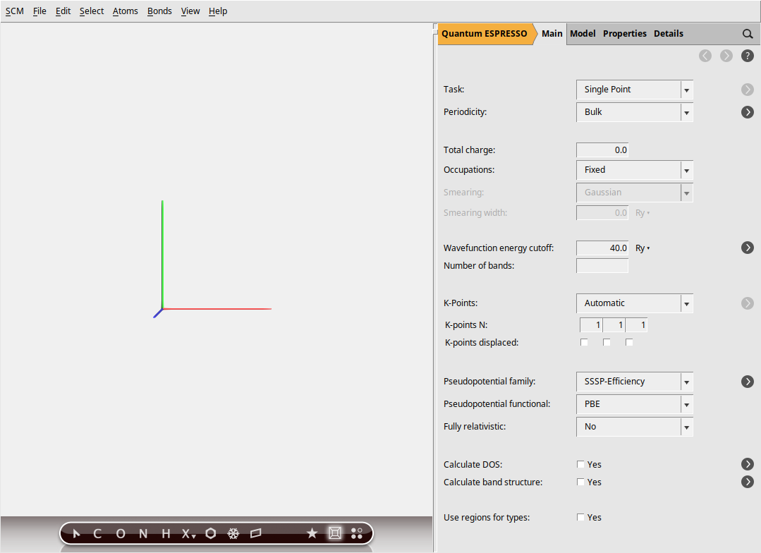
Step 2: Set up the system - Silicon

Copy-paste the coordinates

1. Copy the following coordinates and paste them (ctrl+v) into the molecule-drawing area of AMSinput

Si      -0.67875000      -0.67875000      -0.67875000
Si       0.67875000       0.67875000       0.67875000
VEC1       0.00000000       2.71500000       2.71500000
VEC2       2.71500000       0.00000000       2.71500000
VEC3       2.71500000       2.71500000       0.00000000

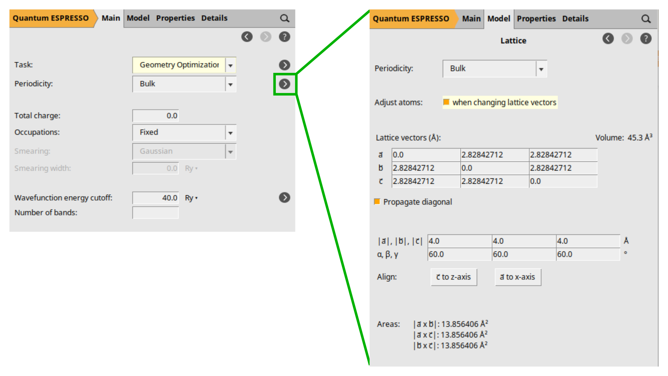
As we want to demonstrate lattice optimization, we will change the lattice a little so something will happen:

1. In the Main panel click the button to the right of the Periodicity option

2. Change all non-zero values in the lattice vectors to 3.0

Step 3: Setting up the calculation

First set up the required geometry optimization:

1. Click on Main to go back to the Main panel

2. Switch the Task to GeometryOptimization

3. Click the button to go to the optimization details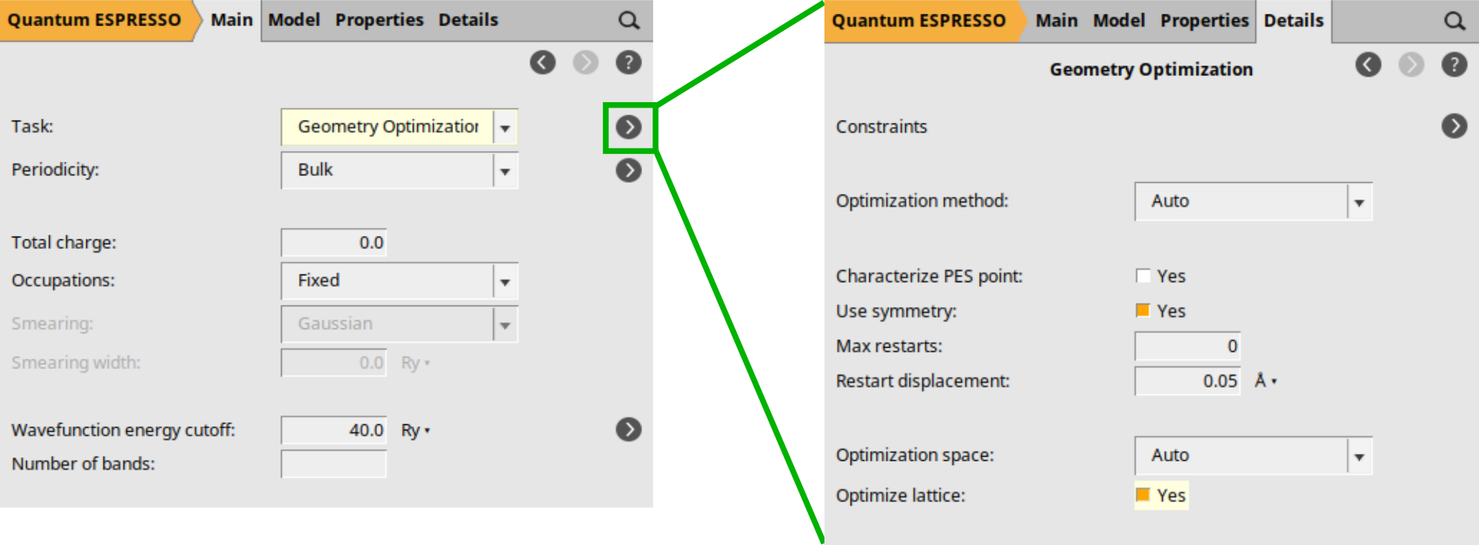

4. Check the Optimize lattice check box

1. Click on Main to go back to the Main panel

We also need to set up the general calculation options.

For this tutorial we will leave most options at their default values.

For real-life application you will have to check if your results are converged with respect to the k-points grid and wavefunction energy cutoff.

Starting with AMS2024, you have the option to use Pseudopotential Families, which significantly simplifies the process of selecting the pseudopotential that best fits your requirements. The three options that follow the Pseudopotentials title work as a filter: all pseudopotentials from the pseudopotential directory that are available for the elements in your system are shown. By choosing options (family, functional, and fully relativistic) you narrow down the list of available pseudopotentials.

If you click on the button located to the right of the Pseudopotentials family, you will be directed to the Pseudopotentials selection details. In this section, you can view the specific UPF file that will be used in the calculation after filtering, along with the recommended minimum energy cutoffs for wave function and density.

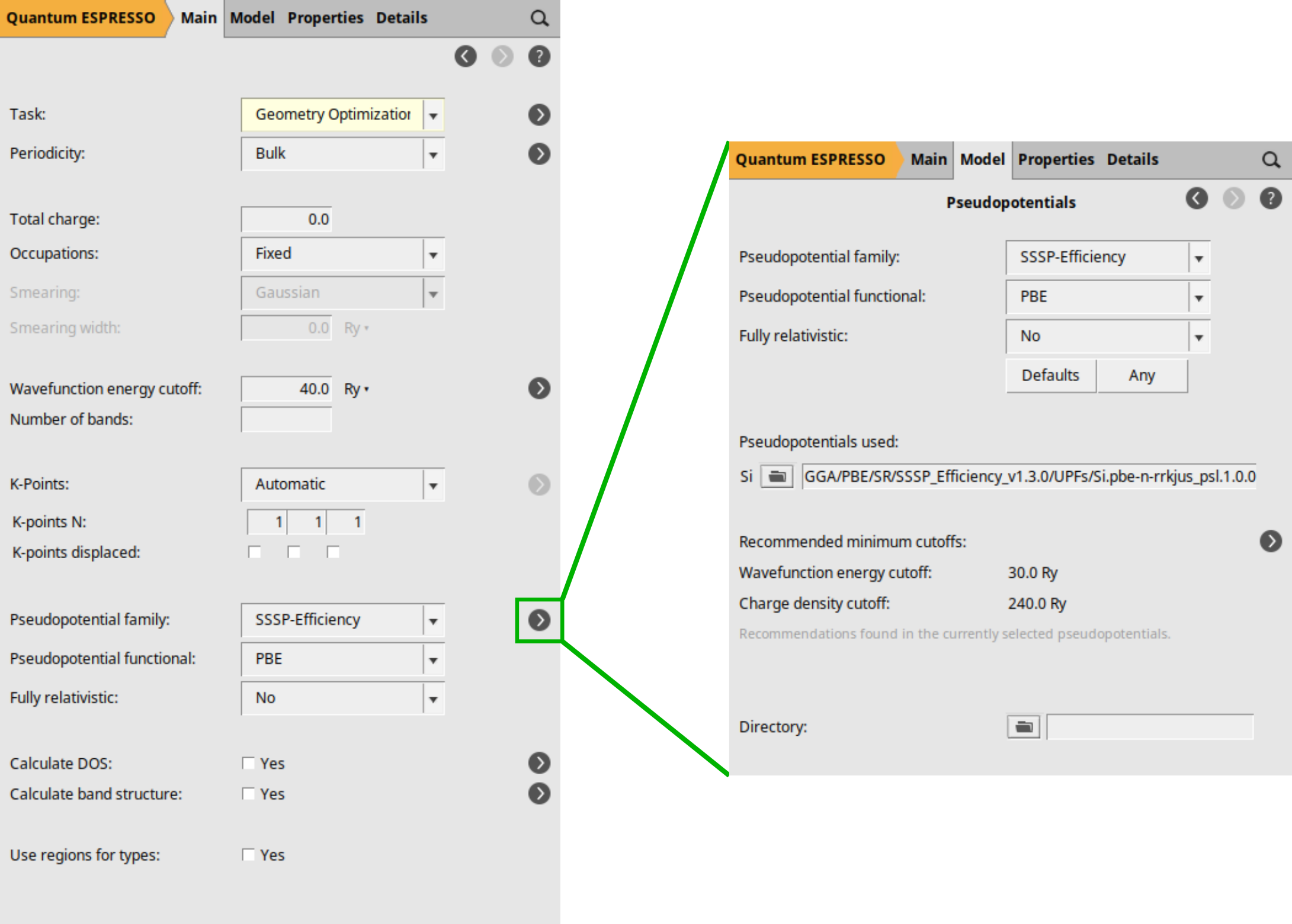
This is just an example, you will need to determine yourself (through calculation and/or literature) which pseudopotentials are best suited for your work.

Finally, set an appropriate k-space sampling (see k-space sampling for some recommendation). In Quantum ESPRESSO, an “automatic” k-point grid means a regular grid (Monkhorst-Pack grid).

1. Set K-points N to 10, 10, 10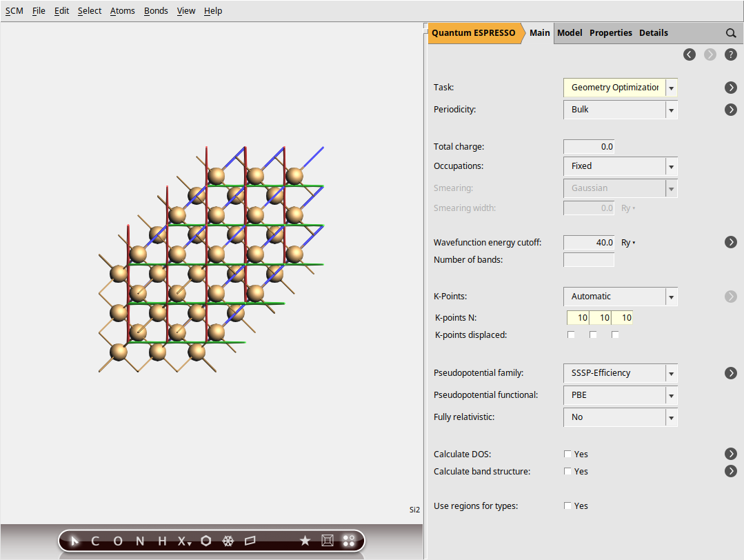

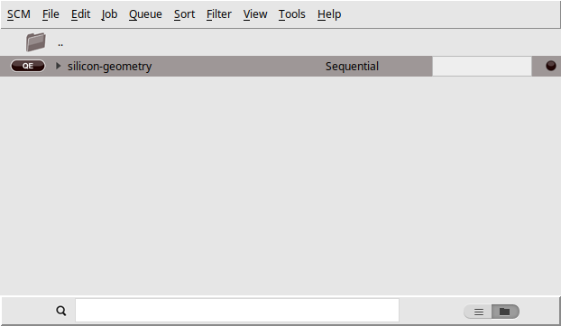
Step 4: Running your job

Running your job on your local machine is very simple:

1. Use the Run command from the File menu: File → Run

2. In the Save File dialog that pops up save your job as silicon-geometry

Your job should start running. In the AMSjobs window you can follow its progress, click on the progress lines to open AMStail showing full details of the progress.

When your job is ready AMSjobs will show this, and AMSinput will prompt you to update the geometry. If you click Yes, New Job the geometry (both the atom coordinates and the lattice vectors) will be updated with the results of your calculation. Now you could continue to perform any other calculation on the optimized system using Quantum ESPRESSO or other AMS engines (like BAND).

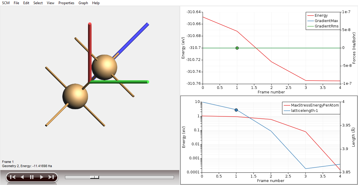
Step 5: Checking the results

At the end of the calculation a .rkf file is automatically created based on the results of Quantum ESPRESSO. RKF files are used by the programs of the AMS suite,

We can now use all the GUI modules to examine the results.

In this tutorial we will have a look at the geometry optimization using AMSmovie:

In AMSjobs

1. Make sure your silicon-geometry job is selected (by clicking on it)

2. Start AMSmovie SCM → Movie

In AMSmovie:

1. Add the length of a lattice vector to the figure: Graph → Lattice Vector Length → Vector 1

2. Click the play button on the left to see the step-by-step progress of the optimization.

Step 6 (optional): Calculating band structure and partial DOS

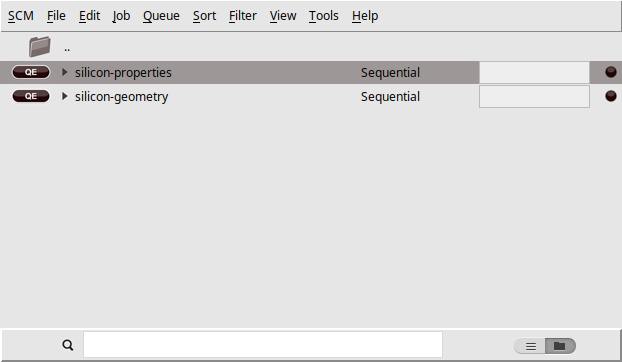
1. Save the job with a another name, for example, silicon-properties: File → Save As…

2. Switch the Task to SinglePoint

3. Set the Number of bands to 8.

4. Check the Calculate DOS and Calculate band structure check boxes.

5. To calculate the partial DOS, click on the button located to the right of the Calculate DOS. you will be directed to the DOS selection details. There, check the Calculate PDOS and Lowdin charges check box.

6. Additionally, to reuse the charge density from our previous geometry optimization, select the generated quantumespresso.rkf file located in the folder named silicon-geometry.results.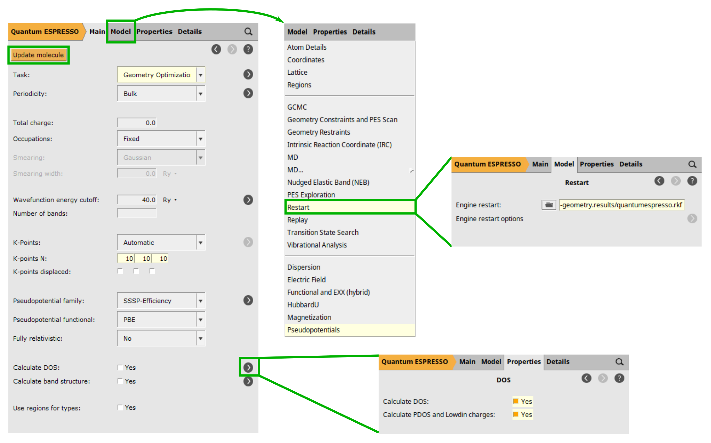 Model → Restart → Engine Restart.

7. Finally, use the Run command from the File menu File → Run to start the calculation.

Your job should start running. In the AMSjobs window you can also follow its progress as in the previous calculation. In the AMSjobs window, note that the job status icon has changed (full circle) to indicate that the job is ready.

Step 7 (optional): Visualizing band structure and partial DOS

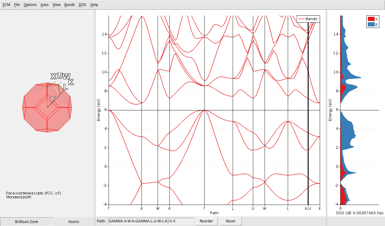
At the end of the calculation, an RKF file is automatically generated based on the Quantum ESPRESSO properties. Now, we can utilize the GUI modules to explore the results. Specifically, we will use AMSbandstructure to visualize the band structure and partial density of states (DOS) by following these steps:

In AMSjobs

1. Make sure your silicon-properties job is selected (by clicking on it)

2. Start AMSbandstructure SCM → Band Structure

The AMSbandstructure window exhibits three linked plots. The left plot illustrates the Brillouin zone (BZ) space, representing the boundaries of the crystal’s unique vectors. The center plot depicts the band structure, where lines delineate the permissible electron energies relative to their wavevector, and the right plot displays the partial density of states (PDOS), featuring distinct curves representing the contributions of various electronic atomic shells to the available energy states.