Quantum ESPRESSO: Magnetism, Band Structure and pDOS
This tutorial will teach you how to:
Set up unrestricted calculations (magnetism) with Quantum ESPRESSO – calculations that allow for different spin configurations on different atoms.
Assign different initial spins – setting a starting point for the magnetic arrangement
Calculate the band structure and DOS in the same job.
Analyze spin results and visualize the band structure and pDOS using AMSoutput, AMSview, and AMSbandstructure.
Our goal is to determine its most stable magnetic configuration by performing Density Functional Theory (DFT) calculations using Quantum ESPRESSO (as an engine) through AMS. We will consider three different states, unpolarized, spin-polarized ferromagnetic, and spin-polarized anti-ferromagnetic, and analyze their respective properties.
Step 1: Start AMSinput
 →
→ 
If you have not yet installed Quantum ESPRESSO a dialog will pop up suggesting to install Quantum ESPRESSO by downloading it from the SCM web site. This is required for this tutorial to work. Downloading may take a while as it is a big package.
If you do not get a popup, you can install Quantum ESPRESSO through the AMS package manager: SCM → Packages
Step 2: Setting up the system
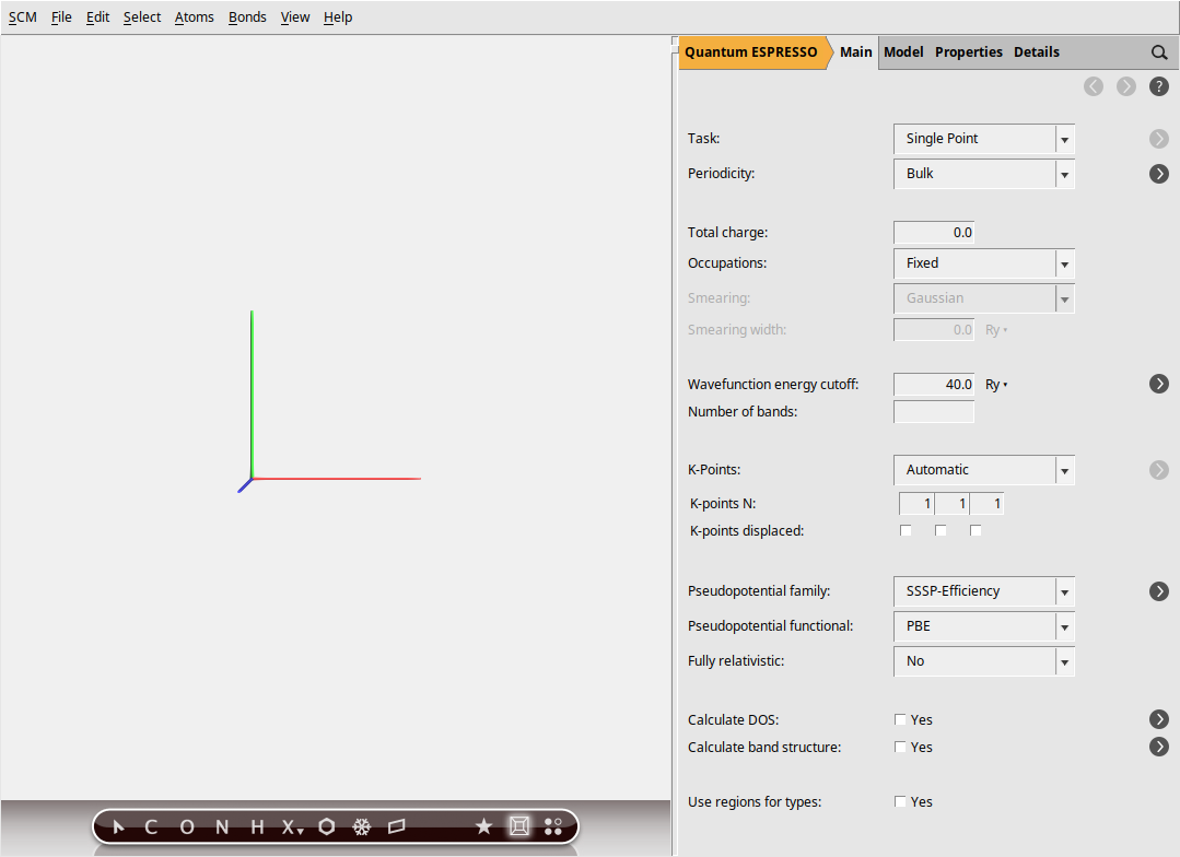
First, create an iron crystal model.

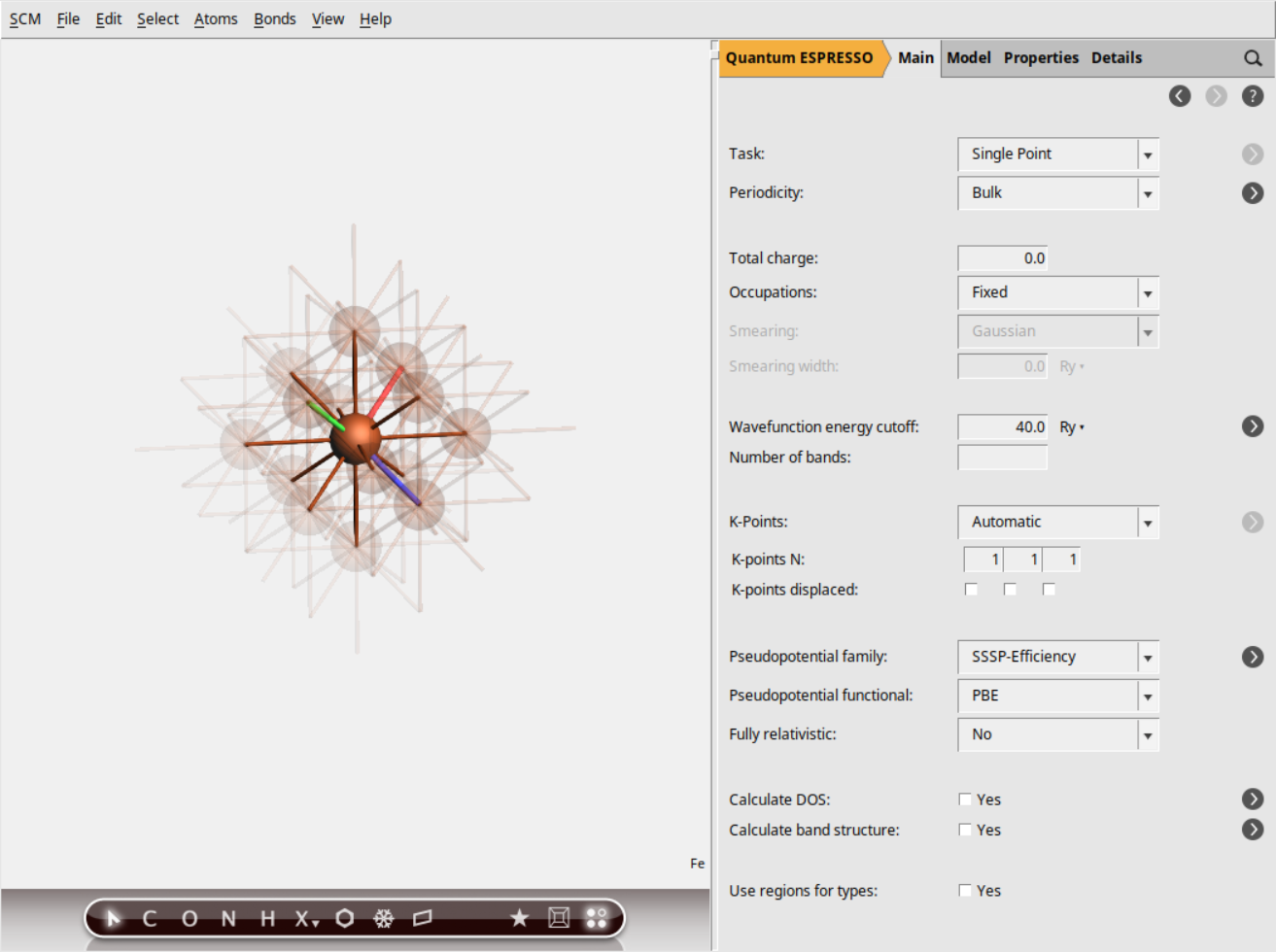
While the unit cell contains a single atom, you can visualize some periodic images for a clearer understanding. Enable periodic visualization and adjust transparency for optimal viewing. Here’s how to do this:
 and then select Complete Molecules. Ensures that some atoms of the periodic structure are also visualized.
Your visualization should now be similar to the following:
Note
This only visualizes some periodic images. It does not create a supercell for the calculation.
Next, we will set up the calculations for our three systems (unpolarized, ferromagnetic, and anti-ferromagnetic) and then move on to executing them.
Step 3: Set up the spin unpolarized calculation
We will begin by calculating the unpolarized ground state of iron. The most simple one. This calculation assumes no net magnetic moment and will provide us with a baseline for comparing different magnetic configurations.
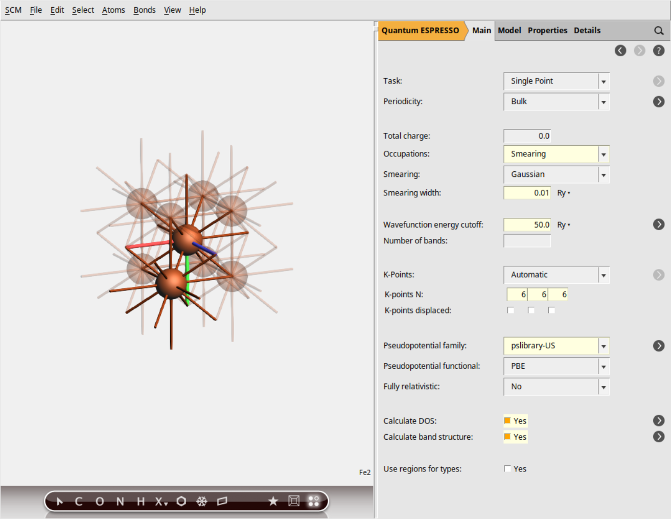
As iron is a metal we will have to use the smearing option. To speed up the calculation, let’s reduce the k-grid to 8x8x8 (for real application you need to test convergence with the k-grid). In this tutorial we will also calculate the pDOS and band structure of the system.
Smearing from the Occupation menu0.01 Ry as smearing width50 Ry.8 8 8 as the number of K points to be usedpslibrary-US from the Pseudopotential family: menu button located to the right of the Calculate DOS: check box
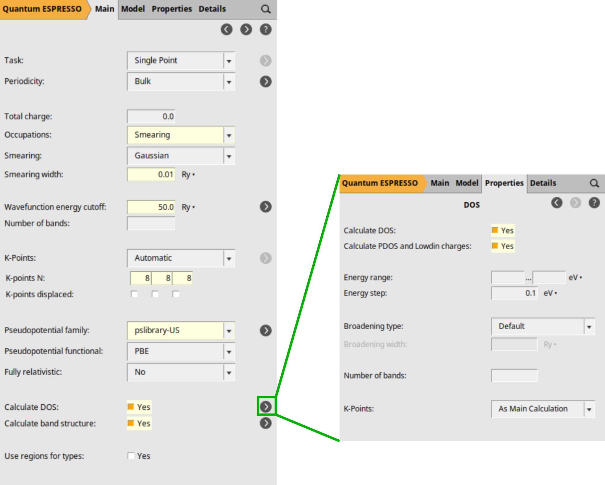
Starting with AMS2024, you have the option to use Pseudopotential Families (see Pseudopotential Families), which significantly simplifies the process of selecting the pseudopotential that best fits your requirements. The three options that follow the Pseudopotentials title work as a filter: all pseudopotentials from the pseudopotential directory that are available for the elements in your system are shown. By choosing options (family, functional, and fully relativistic) you narrow down the list of available pseudopotentials. This is just an example, you will need to determine yourself (through calculation and/or literature) which pseudopotentials are best fit for your work. The choice we make in this tutorial is in no way an advise on which pseudopotential to use, this is just an example.
Tip
Click the next to the wavefunction energy cutoff to see some
recommended settings for the current system and choice of pseudopotentials.
On that panel you can also set the density energy cutoff (ecutrho).
Save your set up as ‘iron-unpolarized’
iron-unpolarized as name and click the Save buttonStep 3: Set up the spin-polarized ferromagnetic calculation
For this system, the changes in the setup are minimal, only the starting magnetization needs to be set differently.
Collinear option1 as the starting magnetization. This initializes the calculation with a spin-polarized configuration.iron-ferromagnetic and click Save.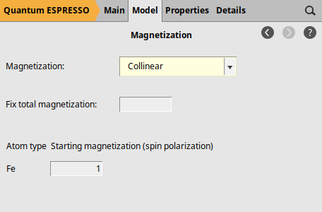
Feel free to try different starting magnetization values and analyze how they impact the results of your spin-polarized calculations. The calculation might find different magnetic ground states (e.g., with varying magnetic moments per atom) depending on the initial guess. This is especially important when the system has multiple possible magnetic configurations. Also, some starting magnetizations might not lead to a stable solution, and the calculation will fail to converge. This can indicate an unphysical starting point or the need to check the calculation setup or convergence criteria. Furthermore, the system might converge to the same magnetic state in some cases regardless of the starting magnetization. This suggests a strong tendency towards that particular magnetic order.
Step 4: Set up the spin-polarized antiferromagnetic calculation
To model the anti-ferromagnetic state of iron, where neighboring atoms have opposite spins, we need to have two atoms in the unit cell. The conventional bcc unit cell of iron has two atoms, so let’s convert the current primitive unit cell to the conventional one:
 and then select Convert To Conventional Cell and then select View Outside Cell (Custom). In the popup window, select 1.2 for View distance outside cell (A):. This ensures that some atoms of the periodic structure are also visualized.
6 6 6 as the number of K points.Please note that we intentionally reduced the number of k-points. This highlights the fact that the conventional cell calculation (super cell) often require fewer k-points than primitive cell calculation to keep the same level of accuracy. However, remember that in real-world applications, it’s crucial to always perform convergence testing with your k-grid to ensure reliable results.
Your visualization should now be similar to the following:
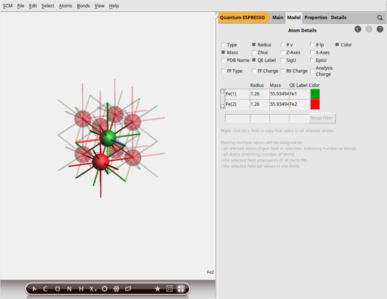
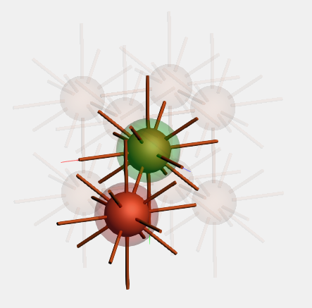
To model anti-ferromagnetic behavior, we need to assign opposite starting spins (“up” and “down”) to our iron atoms. This requires creating two distinct types of iron atoms within the AMS GUI. We can accomplish this using either QE labels (for directly assigning spins to individual atoms) or Regions (for grouping atoms and assigning spins to the whole group). In this tutorial, We will focus on the QE labels method; if you’re interested in learning about the Regions approach, you’ll find a discussion at the end.
Fe1 in the QE Label column. (Optional) Change the Color cell to green (#009e0e) for easier visualization.Fe2 as the QE Label and red (#ff000e) for the Color.You should see distinctly colored atoms (green and red) representing your assigned QE labels (see figure below). You can select multiple atoms simultaneously (using Shift + click) to apply a label to a group, simplifying the process for larger systems. Remember, atoms sharing a QE label will have the same initial magnetization.
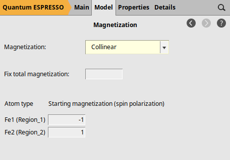
Now, we assign initial magnetization values to the different atom QE labels. To achieve an anti-ferromagnetic configuration, we need to assign one atom label (e.g. Fe1) a starting magnetization of -1 and the other (e.g. Fe2) a starting magnetization of 1. Follow the steps below:
Collinear option is set-1 and 1 as the starting magnetization, respectively.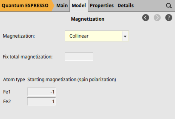
Again, feel free to try different starting magnetization values and analyze how they impact the results of your calculations. Remember that the final SCF calculation may end up in a different state!
Save your set up as ‘iron-antiferromagnetic’
iron-antiferromagnetic as name and click the Save buttonStep 5: Run the calculations
The easy step: use AMSjobs to run your jobs:
You should see the jobs running, one after the other, and you can follow their progress.
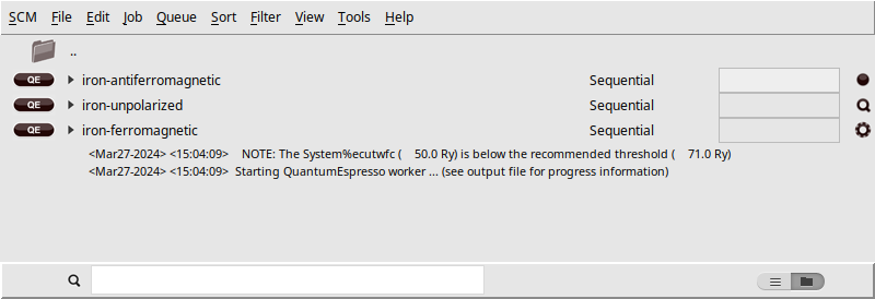
The image above intentionally showcases the calculations in three states, as indicated by the icons on the right-hand side. These icons represent Queued  , Running
  , and Ready
  .
.
Step 6: Examine the results
AMSoutput and AMSview
If you are familiar with Quantum ESPRESSO output, the complete results are available in the AMS output file. A section of particular interest is Lowdin Charges. Depending on your specific calculation, this section shows charges, spin components, and corresponding spin polarizations for each atom and electronic angular momenta. Additionally, AMS conveniently calculates partial charges and adds them at the end. These partial charges reflect the difference between the QE charge and the expected valence electrons based on the pseudopotential used. Note that Löwdin charges are a byproduct of calculating the partial density of states (pDOS). pDOS calculations involve an intermediate step of projecting wavefunctions onto atomic orbitals, and this process also yields the Lowdin charges.
Lowdin: Use the search bar at the bottom of the output window and type Lowdin.The AMSoutput window should automatically scroll to the Lowdin Charges section. You should see something similar to the following figure, which illustrates the output from the antiferromagnetic calculation:
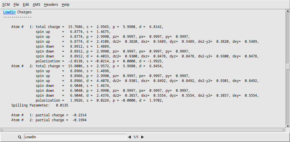
Interestingly, partial Löwdin charges don’t sum to 0.0 (the system’s total charge). This is because Löwdin charges, like other conventional atomic charges, don’t follow strict sum rules. The missing charge can be thought of as a “delocalized” or “bonding” charge (Stefano Baroni, Sept. 2008).
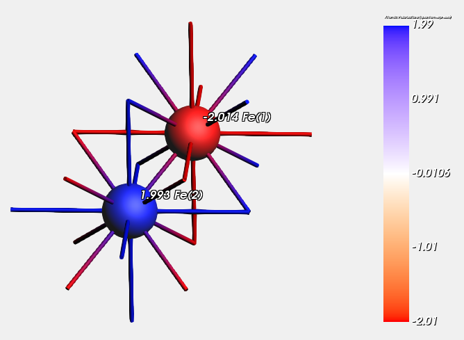
With AMSview you can also examine the atomic properties described above. For example, let’s check the spin:
Now the atomic spins and atom names will be show as a label next the atoms. Even more visual is to color the atoms by the spin:
Moreover, with AMSview you can also visualize fields calculated from the DFT solution. For example, to view the spin polarization density:
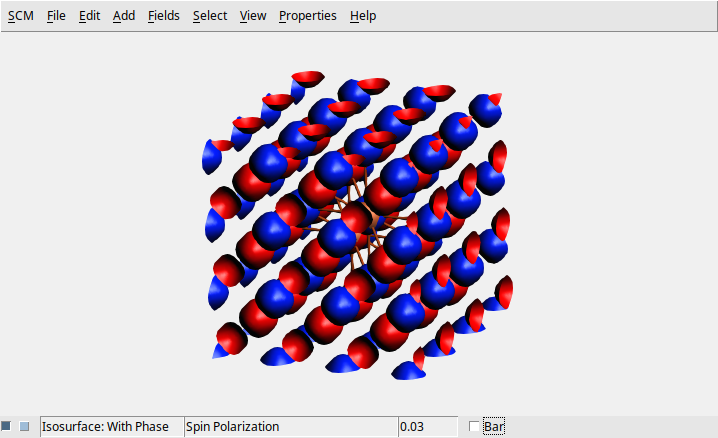
Spin polarization density is particularly interesting because it reveals the difference between up-spin and down-spin electron densities at each point in your material. This information provides key insights into a material’s magnetic behavior, including the type of magnetic ordering and its potential for use in spintronic applications.
Note that in AMSview you can also visualize other field, like the (valence) density and deformation density. Just play with it or check the Advanced AMSview tutorial.
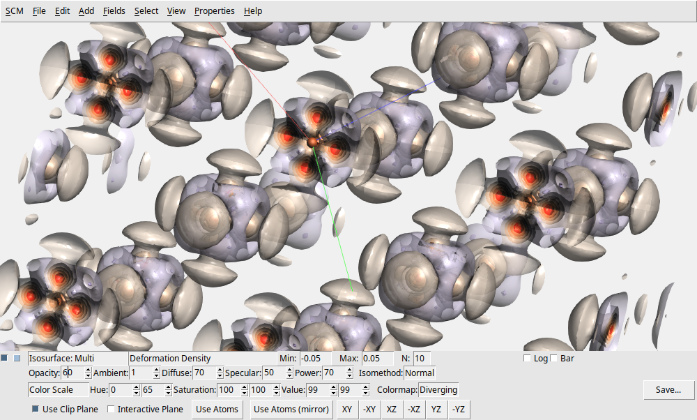
For example, using a multi-iso surface with clip plane and transparency, atoms reduced in size, using a fine grid, you can create the following picture of the deformation density for the spin-polarized state (tip: check the parameters at the bottom of the window):
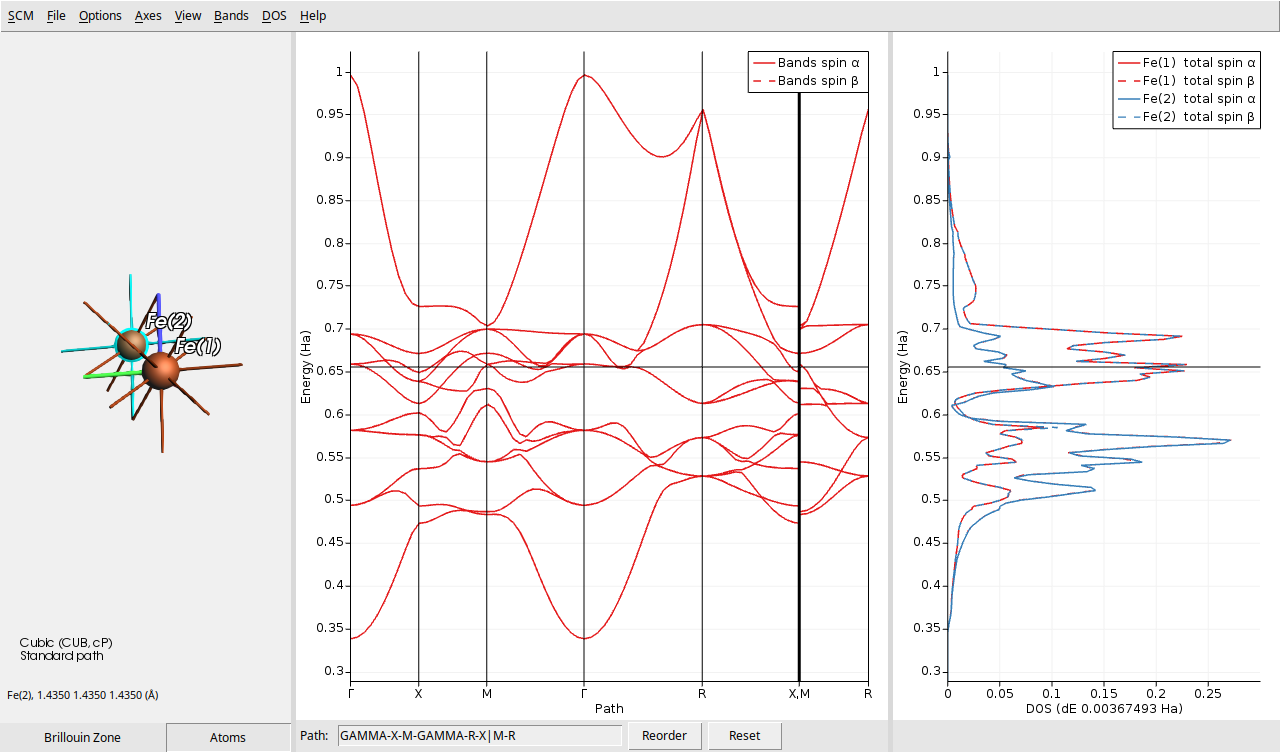
AMSbandstructure
The AMSbandstructure module allows you to analyze various aspects of your system’s electronic structure. If you’ve performed the relevant calculations, you can visualize:
Band structure
Density of States (DOS)
Partial Density of States (pDOS)
Since we have all of these calculations available, let’s dive in and explore them through AMSbandstructure.
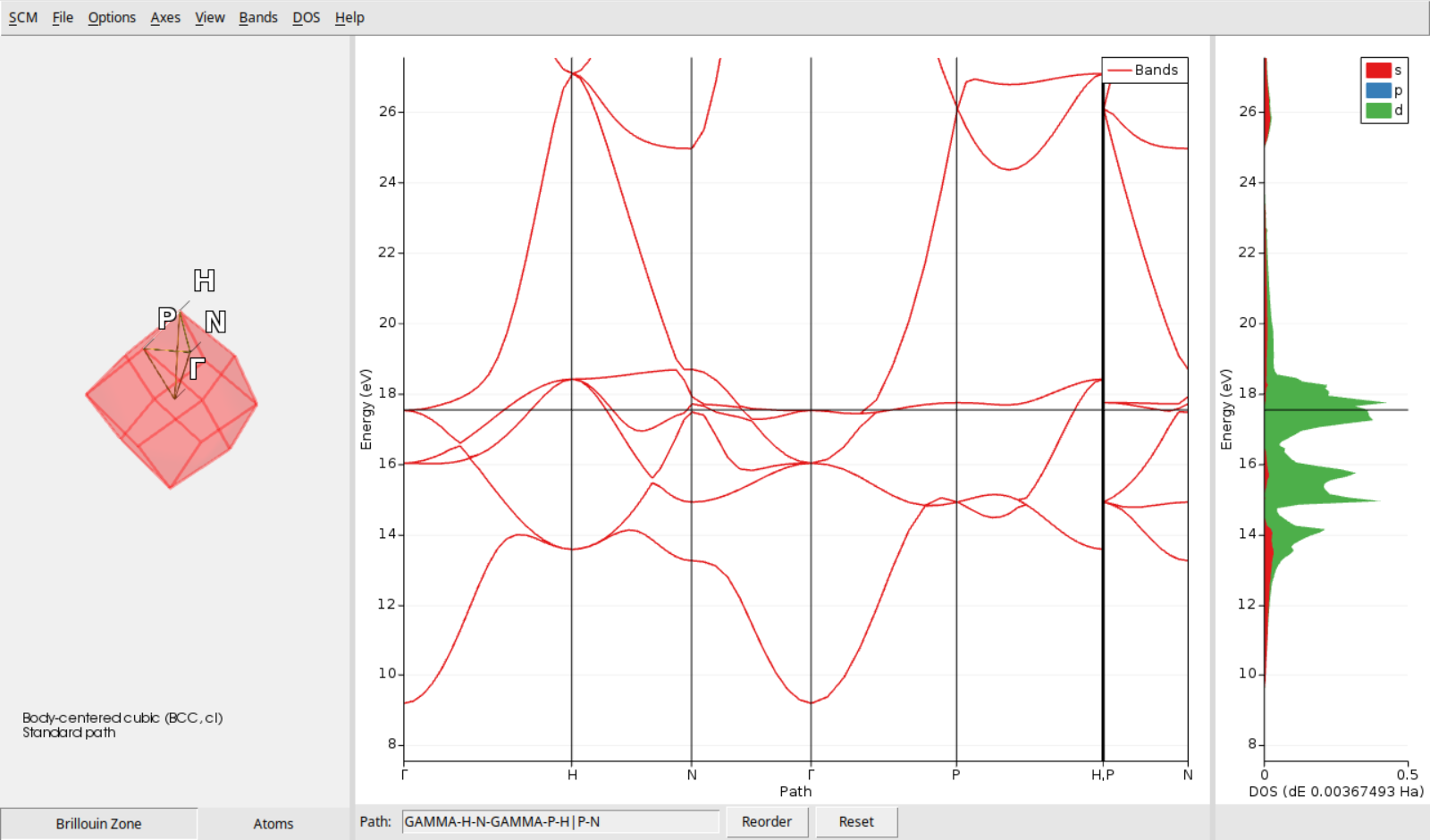
- Unpolarized state
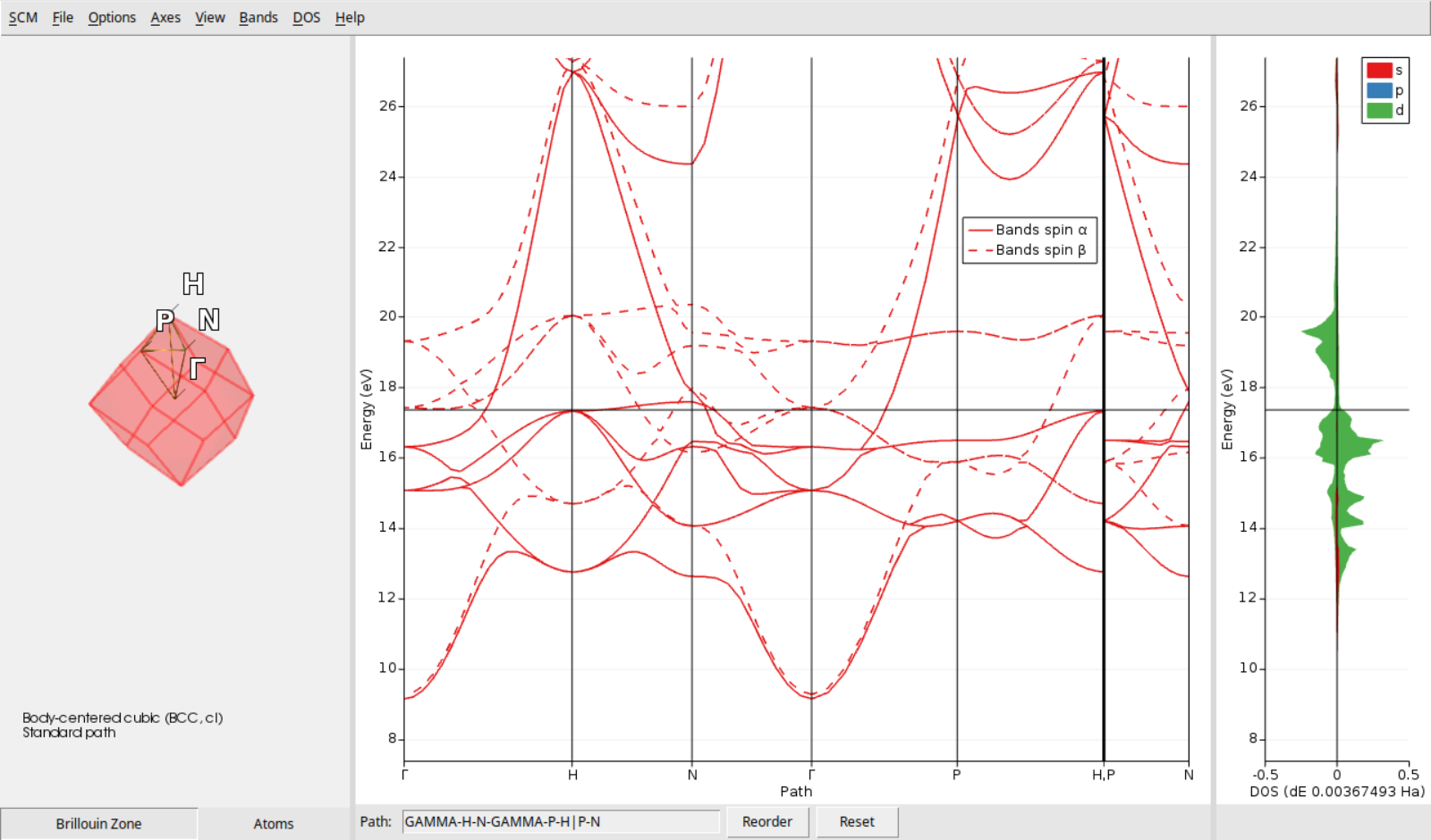
- Spin-polarized state
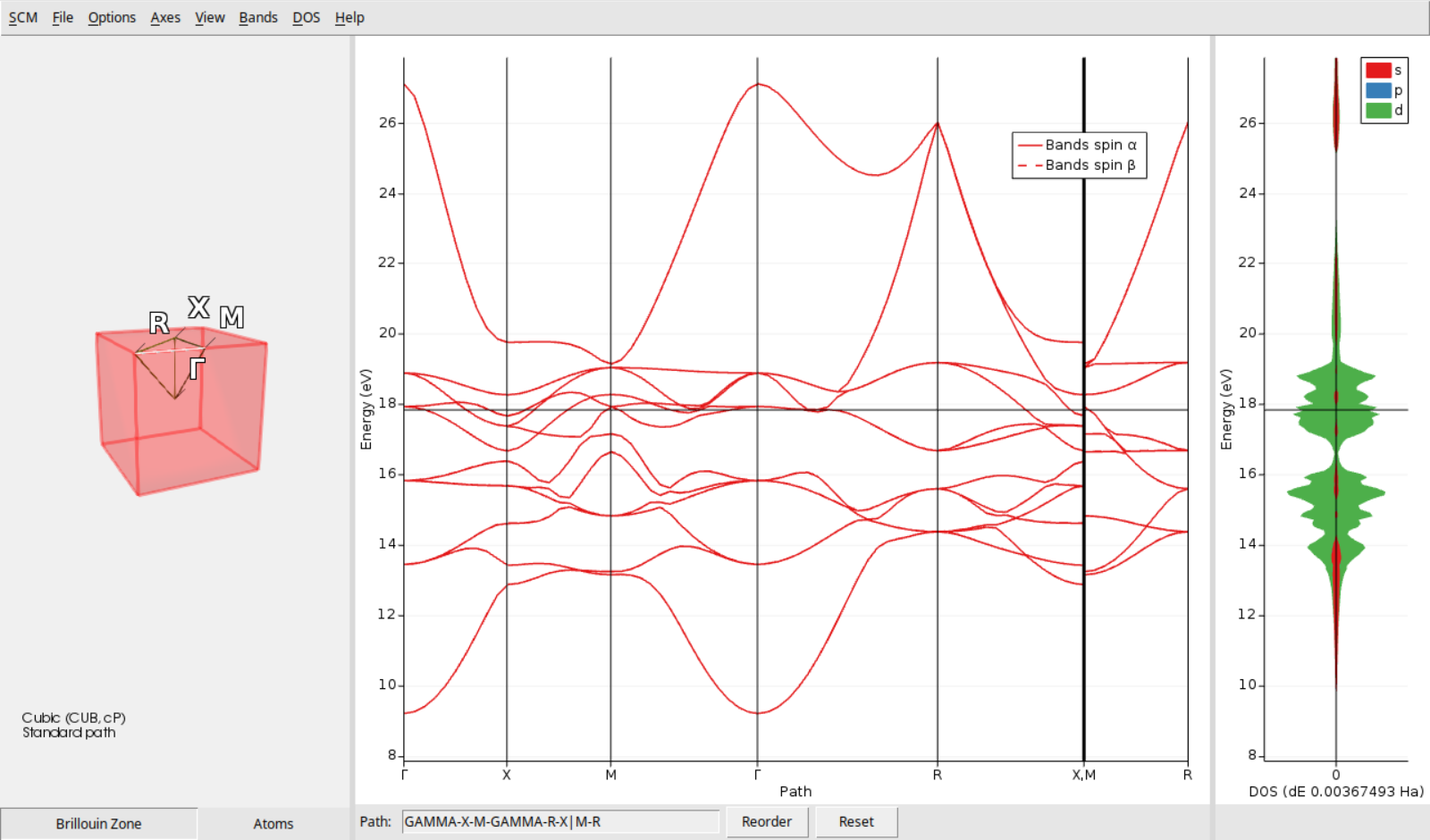
- Anti-ferromagnetic state
Tip
In AMSbandstructure, you can freely move, rotate, and zoom the Brillouin Zone visualization to find the best viewing angle. For finer control, zoom in or out on individual axes on the bands or DOS diagrams by pointing your mouse cursor at the desired axis and using the scroll wheel. Double-click an axis to access its configuration window for even more precise adjustments, like changing ranges or the curves’ colors.
Notice how the alpha and beta band curves overlap in the unpolarized and anti-ferromagnetic cases due to spin symmetry. In contrast, the spin-polarized case reveals distinct structures for the alpha and beta electrons (shown as solid and dotted lines, respectively). Additionally, the partial DOS (pDOS) display allows you to analyze the band composition in terms of atomic shells (s, p, d) for both spins. You can customize the information displayed using the DOS menu.
You can also see the partial DOS for a particular atom:
Tip
In AMSbandstructure, you can change the relative size of the three panels by clicking and dragging the gray line between the panels.
If you look carefully you can see in the DOS section that the spin alpha and beta have been switched for atoms Fe1 and Fe2.
Final note
In this tutorial you did run the Quantum ESPRESSO calculations on your local machine. With AMSjobs you can also run jobs on remote machines. In such cases, AMSoutput, AMSview (for properties), and AMSbandstructure will work naturally as when you ran the calculations in your local machine. You don’t need to transfer your files to your local machine first!
(Optional) Set up the spin-polarized antiferromagnetic calculation via Regions
After converting the crystal to its conventional cell representation (as described in step 4 above), you can easily assign initial spins using Regions instead of QE labels to distinguish between the two types of iron atoms. However, keep in mind, that anyhow the AMS GUI will internally use the QE labels to create the AMS input file.
You should now see something like the following figure. Notice the different colored highlights (red and green); those are your atom regions. For other systems, you can select several atoms at once, holding shift, and put them in the same region. This is important because all the atoms in a region will get the same initial magnetization when we start our calculation.
Now, we assign initial magnetization values to the different atom types (or regions). To achieve an anti-ferromagnetic configuration, we need to assign one atom type a starting magnetization of -1 and the other a starting magnetization of 1. Follow the steps below:
Collinear option is set-1 and 1 as the starting magnetization, respectively.