Quantum ESPRESSO: Phonon Band Structure, DOS, and Thermodynamics¶

Computational Methodology¶

The calculation of phonon properties using Quantum Espresso (QE) involves a series of steps that are handled internally by AMS, making the process transparent to the user. These steps use the QE tools pw.x, ph.x, q2r.x, and matdyn.x. For detailed information about these tools, refer to the official Quantum Espresso documentation online.

Starting from an optimized geometry, we perform a self-consistent field (SCF) calculation using pw.x to determine the electronic ground state of the system. This step solves the Kohn-Sham equations iteratively to obtain the converged electron density and ground state energy, which are essential for subsequent phonon calculations. Next, we use ph.x to calculate the phonon frequencies and eigenvectors at a uniform grid of q-points in the Brillouin zone. This is the most computationally expensive part. This step employs density functional perturbation theory (DFPT) to compute the dynamical matrix, which captures the interatomic force constants and provides the foundation for phonon analysis. Subsequently, q2r.x is used to perform a Fourier transform of the interatomic force constants from the q-point grid to real space, enabling the calculation of phonon properties in a more convenient representation. Finally, matdyn.x is employed to post-process the phonon data, allowing us to extract the phonon DOS and band structure (these are two independent calculations). This step involves calculating phonon frequencies for arbitrary q-vectors, including those along high-symmetry paths, using the interatomic force constants obtained from the dynamical matrices.

Once the phonon DOS \(D_p(\varepsilon)\) is calculated, we can determine various thermodynamic properties using the canonical distribution from statistical mechanics for phonons under the harmonic approximation. These properties are crucial for analyzing the thermal behavior of materials.

In AMS, thermodynamic properties are automatically calculated when the DOS is requested, offering a convenient way to access this information. The properties derived from the phonon DOS are calculated as follows:

• Internal energy (\(U\)): Represents the total energy of the system due to phonons.

• Specific heat (\(C_V\)): Measures the amount of heat required to raise the temperature of the material by a certain amount at constant volume.

• Helmholtz free energy: (\(F\)): Represents the thermodynamic potential that measures the useful work obtainable from a closed system at a constant temperature and volume.

• Entropy (\(S\)): Measures the degree of disorder or randomness in the system.

These thermodynamic properties provide a comprehensive picture of the thermal behavior of materials and are crucial for understanding and predicting their response to temperature changes. This information is particularly important for various applications, such as designing efficient heat sinks, thermal barrier coatings, and for understanding the stability and phase transitions of materials at different temperatures.

The phonons properties can be calculated using Quantum Espresso through AMS via two main interfaces: the graphical user interface (GUI) and the Python library, PLAMS. The GUI presents a user-friendly, visual approach that is ideal for users performing routine calculations on simple systems. It simplifies the process of setting up input files and visualizing results. On the other hand, PLAMS offers a powerful and flexible Python environment suitable for complex workflows, parameter sweeps, and integration with other scientific libraries. This makes it particularly advantageous for advanced users, high-throughput calculations, or situations that require automation and scripting, providing greater control and customization of the computational process. In this tutorial, we will explore both options. They are completely independent, so you can jump directly to the section that interests you the most.

Using the GUI¶

We will use the following structure as basis for the subsequent calculations:

Be       0.0000000000       1.5555413800       0.0007009000
Be       1.3471383600       0.7777706900       2.1887103500
 O       0.0000000000       1.5555413800       1.6512462200
 O       1.3471383600       0.7777706900       3.8392556700
VEC1    2.6942767100     0.0000000000     0.0000000000
VEC2   -1.3471383600     2.3333120800     0.0000000000
VEC3    0.0000000000     0.0000000000     4.3760188900

Setting Up the Calculation:

1. Open AMSinput

2. Copy & paste the coordinates above into AMSinput.

3. Switch to

4. Select Task → GeometryOptimization

5. Change the Wavefunction energy cutoff to 25 Ryd

6. Change the K-Points N to 4 4 3

You should get something like this:

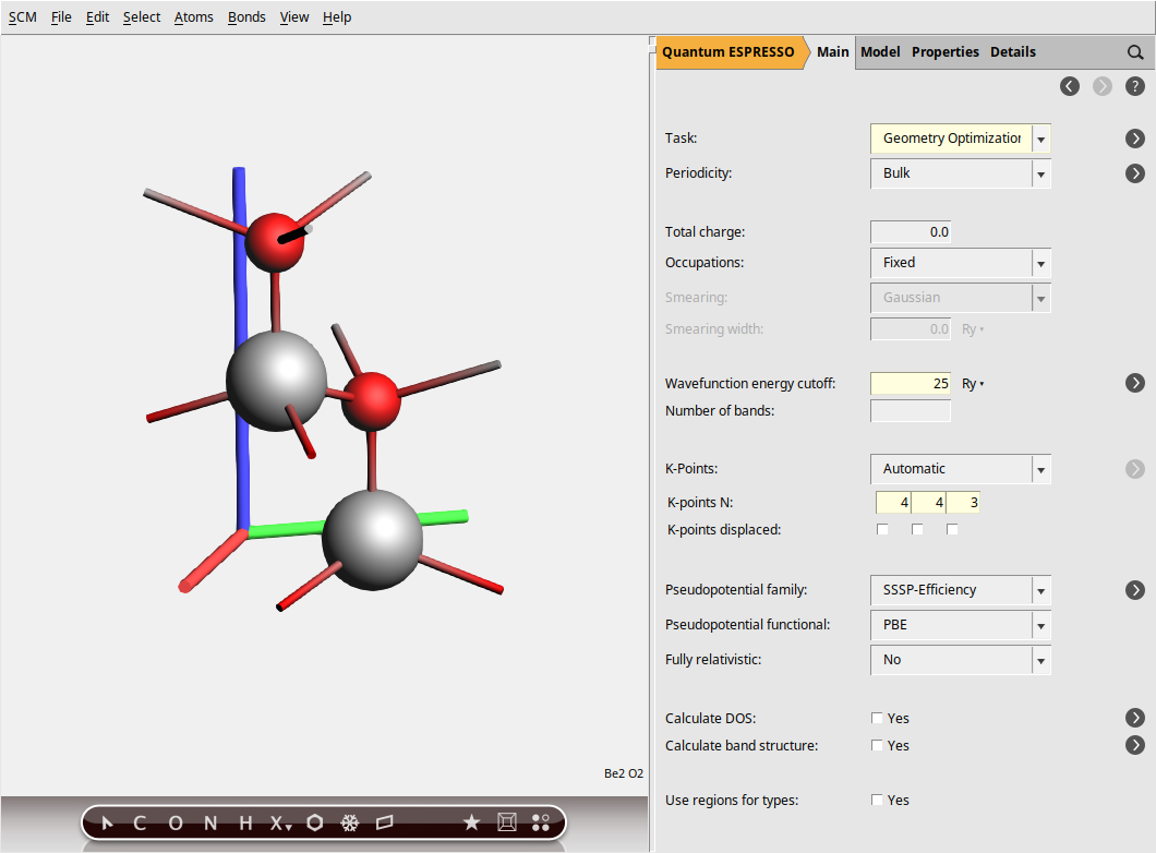
In the steps above, we specified a GeometryOptimization task to ensure our BeO structure is at a local energy minimum, preventing any spurious imaginary frequencies in the phonon spectrum. Next, for the electronic structure part, we set the plane-wave energy cutoff (ecutwfc) to 25 Ry. While this value is lower than typically recommended for production calculations (40 Ry), we use it here for demonstration purposes to reduce computational cost. Then, the Brillouin zone sampling is done using a Monkhorst-Pack k-point grid of size 4 × 4 × 3, ensuring a balanced sampling in all directions.

Now, use the panel bar Properties → Phonons and Elastic Tensor command to go to the Phonons (and Elastic Tensor) configuration panel. Then:

1. Activate the calculation of phonons by checking Yes in the Phonons check box.

2. Click the next to the Method entry to configure the details of the Analytical Phonons calculation.

3. Change the number of q-points to use in the entry Q-Points N: to 4, 4, 3 to use a Monkhorst-Pack q-point grid of size 4 x 4 x 3.

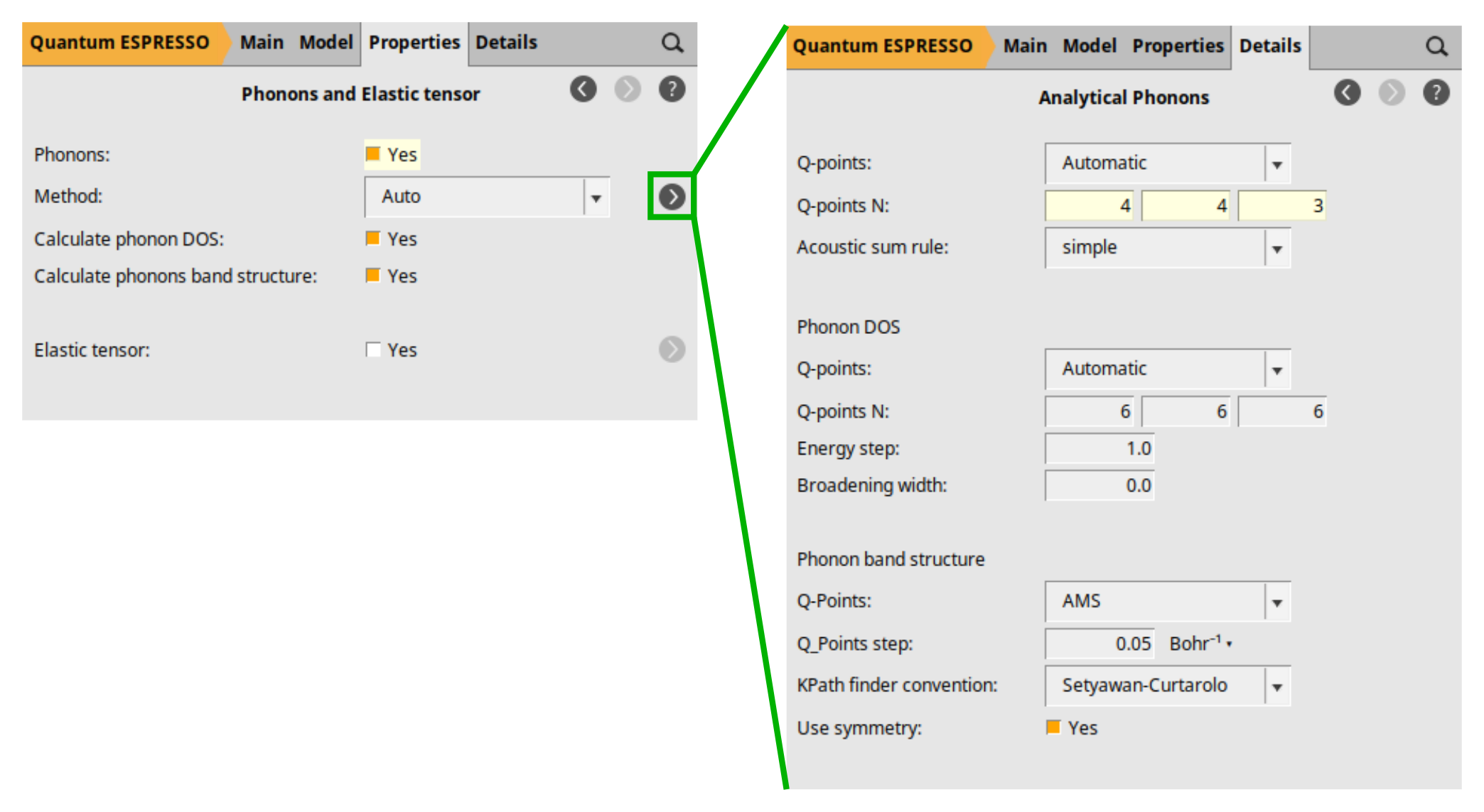
Here, we activated the calculation of phonons (Phonons: Yes), which by default calculates both the phonon band structure and the DOS. Notice the checkboxes Calculate phonon DOS and Calculate phonons band structure. We defined a 4 × 4 × 3 q-point grid for our phonons calculation. A coarser q-point grid is normally preferred to the k-point grid (electronic part), as phonon calculations are more computationally intensive. However, the right choice should be obtained by a convergence test. AMS uses the specified q-grid for the initial analytical calculation of phonon frequencies within Quantum Espresso. However, the band structure plot is generated by interpolating those frequencies onto a denser set of q-points along the high-symmetry path proposed by Setyawan and Curtarolo. You can change the path convention using the dropdown list KPath finder convention:. This interpolation scheme, using a Fourier interpolation, allows for the construction of continuous phonon dispersion curves, providing a clearer visualization of the phonon band structure and facilitating the analysis of vibrational frequencies across different regions of the reciprocal space.

Computation & Results¶

We are now ready to start the calculation

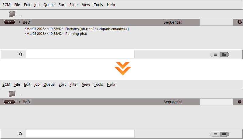
1. Select File → Save As and give it an appropriate name (e.g. BeO)

2. Select File → Run

3. Wait for the calculation to finish (this should take a few minutes). Click Yes when asked to load the optimized geometry in AMSinput.

When you run a calculation, AMSjobs should come to the forefront, and your job will appear at the top of the list. On the right side, you’ll see the job running, indicated by a gear icon. While the simulation is in progress, the AMSjobs window will display the progress based on the logfile. Once the job is complete, the job status icon will change to a full circle to indicate that it is ready.

The AMSband module allows you to analyze both the Band structure and the DOS. Both properties are widely used because they reveals key features such as the distinction between acoustic and optical modes, the dispersion and anisotropy of phonon frequencies, the presence of frequency gaps, and the distribution of vibrational modes.

In AMSjobs (with your job selected) or AMSinput

Start the AMSband module by clicking (SCM → Band Structure)

You should get the following:

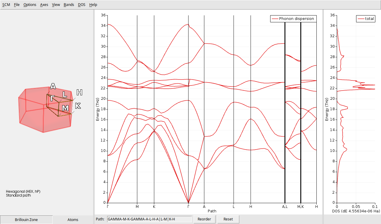
AMSbands provides a summarized view of the vibrational properties of BeO. On the left side, there is a visual representation of the first Brillouin zone. In the central section, you can see the phonon band structure, while the right side displays the DOS.

The Brillouin zone of BeO, shown on the left, reflects its hexagonal wurtzite crystal structure. Focusing on the central portion, the red lines indicate the dispersion of phonon frequencies across different high-symmetry directions in the Brillouin zone. Distinct branches correspond to acoustic and optical phonon modes: acoustic modes approach zero frequency at the center (\(\Gamma\) point), while optical modes exhibit non-zero frequencies. The right panel illustrates the phonon DOS, which indicates the number of vibrational modes at each frequency. Peaks in the DOS correspond to regions with a high density of phonon modes.

These combined plots offers insights into how phonon frequencies vary with the wave vector, highlights the dominant vibrational frequencies, and reveals the presence of any gaps or degeneracies in the phonon spectrum.

Theoretical results for comparison can be found in The Computational Raman Database (mpid: mp-2542).

Tip

In AMSbandstructure, you can freely move, rotate, and zoom the Brillouin Zone visualization to find the best viewing angle. For finer control, zoom in or out on individual axes on the bands or DOS diagrams by pointing your mouse cursor at the desired axis and using the scroll wheel. Double-click an axis to access its configuration window for even more precise adjustments, like changing ranges or the curves’ colors.

Tip

In AMSbandstructure, you can change the relative size of the three panels by clicking and dragging the gray line between the panels.

The AMSdos module allows you to focus on the DOS.

In AMSjobs (with your job selected) or AMSinput

Start the AMSdos module by clicking (SCM → Dos)

You should get the following:

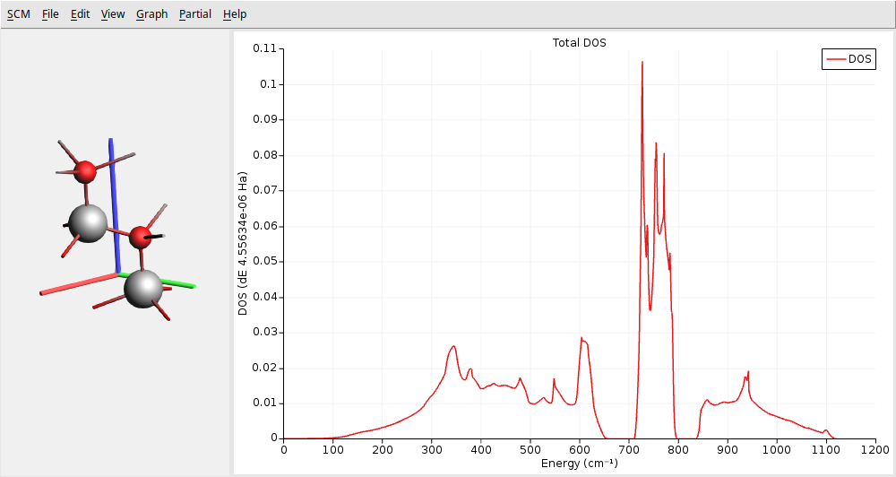
This figure shows three distinct regions separated by two gaps. At lower frequencies, the first region typically has contributions from acoustic and optical modes (confirmed with the phonon band structure above). Optical modes primarily dominate the second and third regions. In particular, we can see the intense characteristic peak associated with wurtzite structures around \(650 \text{cm}^{-1}\). This peak is mainly attributed to the \(E^2_h\) optical phonon mode, which is quite flat in the band structure. This mode involves vibrations perpendicular to the c-axis and is exclusively Raman-active.

After examining the phonon band structure and the DOS, we will now focus on the thermodynamic properties derived from the latter, as described at the beginning of this tutorial. To do this, we will use the KFBrowser tool:

In AMSjobs (with your job selected) or AMSinput

Start the KFBrowser module by clicking (SCM → KF Browser)

Then click on (File → Related Files → quantumespresso.rkf)

Finally, click on the small black triangle close to the Plots section.

KFBrowser allows you to explore all the data stored in the binary files ams.rkf (specific to AMS) and engine.rkf (specific to the engine). It contains all the information considered important during the entire calculation, such as energies, geometries, gradients, and in this case, the thermodynamic properties of the phonons. Following the instructions above, you will open the engine file quantumespresso.rkf, which should appear as follows:

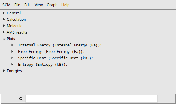
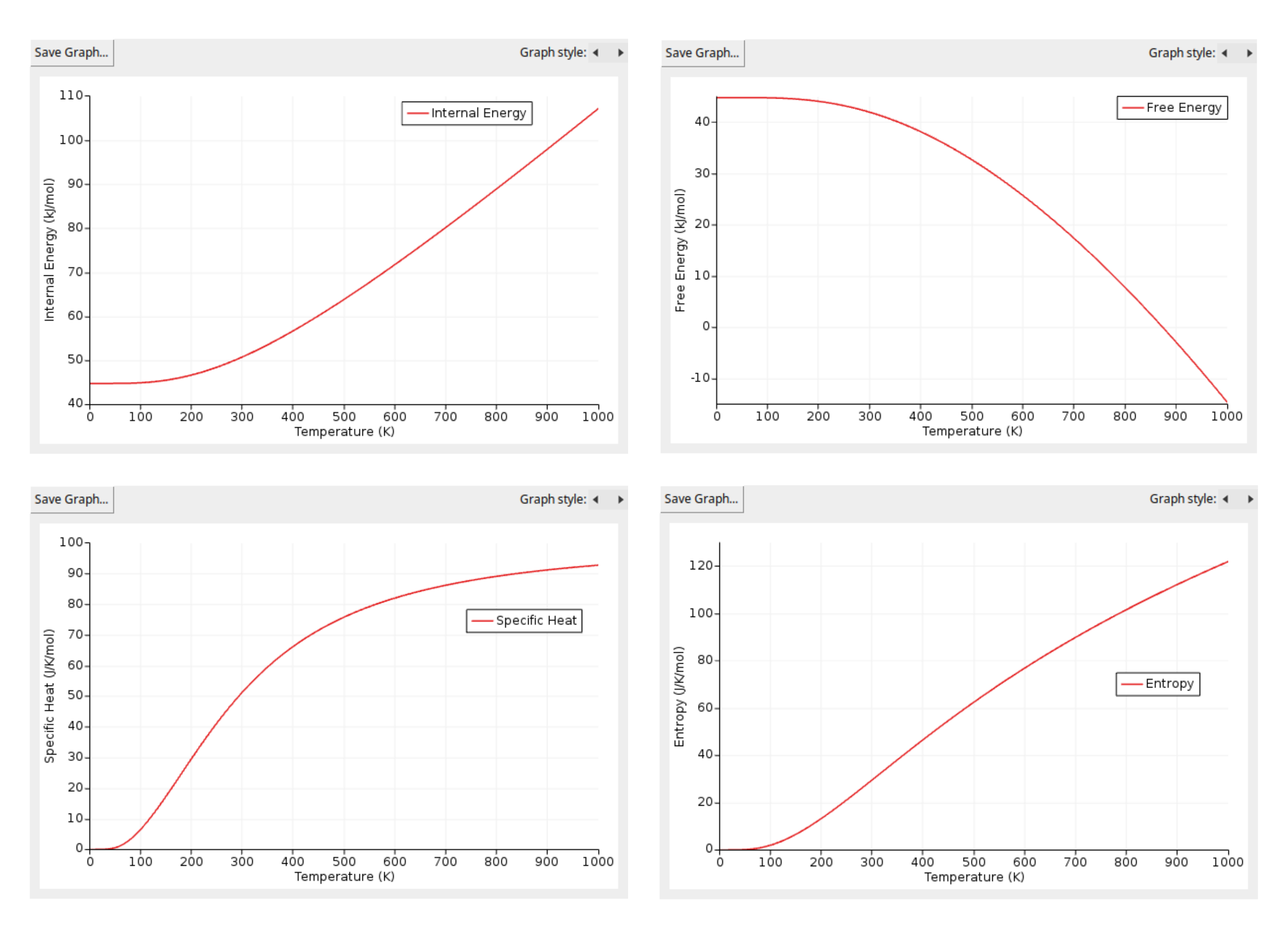
In the Plots section, you will find four thermodynamic properties: internal energy, free energy, specific heat, and entropy. You can generate a clear figure for each property by simply double-clicking on the one you are interested in. The figures you should obtain are the following:

Tip

In these plots, double-click on the y-axis to change the units, for example, from Hartree to kJ/mol for internal energy and free energy, or from kB (Boltzmann constant units) to J/K/mol.

These figures illustrate the calculated thermodynamic properties of BeO as a function of temperature, derived from the phonon DOS. From them, we can see a couple of interesting features:

Firstly, the internal energy (\(U\)) increases steadily with temperature, starting from the Zero Point Energy (ZPE) at 0 K (44.70 kJ/mol). This trend aligns with the increase in vibrational energy of the atoms as the temperature rises.

Secondly, the specific heat (\(C_v\)) exhibits a characteristic behavior commonly observed in many solids. It increases rapidly at low temperatures due to the gradual excitation of vibrational modes. As the temperature continues to rise, the specific heat approaches a plateau known as the Dulong-Petit limit. This limit represents the classical regime in which all vibrational modes are fully excited. For BeO, our calculations indicate that the Dulong-Petit limit is approximately 99.77 J/K/mol of unit cells, which corresponds to 3n*R, where n is the number of atoms per unit cell and R is the ideal gas constant. To express this limit per mole of atoms, as is traditionally done, we divide by n to arrive at the well-known value of 3R.

Using Python (PLAMS)¶

To start, we import the matplotlib library, which is essential for visualizing different aspects of our calculations, such as molecular geometry, as well as the resulting phonon properties. By setting plt.rcParams['figure.dpi'] = 120, we adjust the resolution of the figures to ensure they are displayed with sufficient clarity and detail.

import matplotlib.pyplot as plt
plt.rcParams['figure.dpi'] = 120

As previously mentioned, we use the PLAMS Python library to interact with AMS. The code below constructs the beryllium oxide (BeO) crystal structure by defining a Molecule object. Individual atoms, beryllium (Be) and oxygen (O), are then added to the molecule using their respective symbols and Cartesian coordinates, which are specified in Angstroms. Next, the crystal lattice is defined as a 3x3 matrix, with dimensions also in Angstroms.

from scm.plams import Molecule, Atom, plot_molecule

mol = Molecule()
mol.add_atom(Atom(symbol="Be", coords=(0.00000000, 1.55554138, 0.00070090)))
mol.add_atom(Atom(symbol="Be", coords=(1.34713836, 0.77777069, 2.18871035)))
mol.add_atom(Atom(symbol= "O", coords=(0.00000000, 1.55554138, 1.65124622)))
mol.add_atom(Atom(symbol= "O", coords=(1.34713836, 0.77777069, 3.83925567)))
mol.lattice = [[ 2.69427671, 0.00000000, 0.00000000], \
               [-1.34713836, 2.33331208, 0.00000000], \
               [ 0.00000000, 0.00000000, 4.37601889]]

To visualize the BeO crystal structure we’ve defined, we employ the plot_molecule function. This function serves as an interface to the plot_atoms function from the Atomic Simulation Environment (ASE), enabling us to generate graphical representations of the atomic arrangement. For a more detailed control over the generated figures, you can consult the original ASE documentation. In this particular instance, we generate three distinct views of the BeO structure by applying different rotation angles. Specifically, we create a figure with three subplots, each displaying the molecule rotated along different axes: ('15x,15y,0z'), ('0x,90y,0z'), and ('0x,0y,0z').

fig, ax_arr = plt.subplots(1, 3)
ax_arr[0] = plot_molecule(mol, ax=ax_arr[0], rotation=('15x,15y,0z'))
ax_arr[1] = plot_molecule(mol, ax=ax_arr[1], rotation=('0x,90y,0z'))
ax_arr[2] = plot_molecule(mol, ax=ax_arr[2], rotation=('0x,0y,0z'))

To set up the Quantum Espresso phonon calculation, we first create a Settings object in PLAMS to store all the calculation parameters. We begin by specifying a GeometryOptimization task to ensure our BeO structure is at a local energy minimum, preventing any spurious imaginary frequencies in the phonon spectrum. Next, we activate the calculation of phonons (Properties%Phonons = Yes), which will provide us with the phonon band structure and density of states (DOS).

For the electronic structure part, we set the plane-wave energy cutoff (ecutwfc) to 25 Ry. While this value is lower than typically recommended for production calculations (40 Ry), we use it here for demonstration purposes to reduce computational cost. The Brillouin zone sampling is done using a Monkhorst-Pack k-point grid of size 4 × 4 × 3, ensuring a balanced sampling in all directions. Additionally, we also use a 4 × 4 × 3 q-point grid for our phonons calculation. A coarser q-point grid is normally preferred to the k-point grid (electronic part), as phonon calculations are more computationally intensive. However, the right choice should be obtained by a convergence test.

AMS uses the specified q-grid for the initial analytical calculation of phonon frequencies within Quantum Espresso. However, the band structure plot is generated by interpolating those frequencies onto a denser set of q-points along the high-symmetry path proposed by Setyawan and Curtarolo (convention Phonons%BandStructure%KPathFinderConvention = 'Setyawan-Curtarolo'). This interpolation scheme, using a Fourier interpolation, allows for the construction of continuous phonon dispersion curves, providing a clearer visualization of the phonon band structure and facilitating the analysis of vibrational modes across different regions of the reciprocal space.

The pseudopotentials used in this calculation are based on the SSSP-Efficiency family with the PBE functional and no relativistic corrections, as this is the default choice in AMS. Finally, we create an AMSJob object named "BeO" that combines the settings and the previously defined BeO molecule, encapsulating all the information needed to run the Quantum Espresso calculation.

from scm.plams import Settings, AMSJob

s = Settings()
s.input.ams.Task = "GeometryOptimization"
s.input.ams.Properties.Phonons = "Yes"
s.input.QuantumEspresso.System.ecutwfc = 25.0
s.input.QuantumEspresso.K_Points._h = "automatic"
s.input.QuantumEspresso.K_Points._1 = "4 4 3 0 0 0"
s.input.QuantumEspresso.Phonons.Q_Points._h = "automatic"
s.input.QuantumEspresso.Phonons.Q_Points._1 = "4 4 3 0 0 0"

job = AMSJob(settings=s, molecule=mol, name="BeO")

The job.get_input() function retrieves the content of the AMS input file generated during the previous setup. This enables users to inspect the input parameters before running the Quantum Espresso calculation. Reviewing the input file can be beneficial for advanced users who seek greater control over the calculation settings.

print(job.get_input())

Properties
  Phonons Yes
End

Task GeometryOptimization

System
  Atoms
             Be       0.0000000000       1.5555413800       0.0007009000
             Be       1.3471383600       0.7777706900       2.1887103500
              O       0.0000000000       1.5555413800       1.6512462200
              O       1.3471383600       0.7777706900       3.8392556700
  End
  Lattice
         2.6942767100     0.0000000000     0.0000000000
        -1.3471383600     2.3333120800     0.0000000000
         0.0000000000     0.0000000000     4.3760188900
  End
End

Engine QuantumEspresso
  K_Points automatic
     4 4 3 0 0 0
  End
  Phonons
    Q_Points automatic
       4 4 3 0 0 0
    End
  End
  System
    ecutwfc 25.0
  End
EndEngine

We call the run() method on the previously defined AMSJob object to start the Quantum Espresso calculation. This starts the execution of the job, and once it is completed, the results are stored in the results object. The output displays various stages of the job’s progress, including STARTED, RUNNING, FINISHED, and finally, SUCCESSFUL, which indicates that the calculation has been completed without any errors.

results = job.run()

[27.03|10:20:29] JOB BeO STARTED
[27.03|10:20:29] JOB BeO RUNNING
[27.03|10:26:38] JOB BeO FINISHED
[27.03|10:26:38] JOB BeO SUCCESSFUL

The phonon band structure is widely used because it provides a clear understanding of how vibrational modes (phonons) propagate and interact within a crystalline material.

To visualize the phonon band structure, we can use the plot_phonons_band_structure function provided by PLAMS. This function takes the phonon band structure data, which we can obtain from the results object using the get_phonons_band_structure method, and generates a plot of the phonon frequencies along the specified high-symmetry path in the Brillouin zone. The unit="cm^-1" argument ensures that the frequencies are displayed in units of wavenumbers.

The plot_phonons_band_structure function uses matplotlib for plotting, so we can further customize the plot using matplotlib’s functionalities. In this case, we set the y-axis and x-axis labels, and the title of the plot. This plot provides a visual representation of the phonon band structure, allowing us to analyze the dispersion of phonon frequencies across the Brillouin zone and identify key features such as acoustic and optical modes, band gaps, and degeneracies.

from scm.plams import plot_phonons_band_structure

phonons_data = results.get_phonons_band_structure(unit="cm^-1")
ax = plot_phonons_band_structure(*phonons_data)

ax.set_ylabel("Frequency (cm$^{-1}$)")
ax.set_xlabel("Wave Vector")
ax.set_title("BeO Phonons")

plt.show()

The image displays a comprehensive view of the vibrational properties of BeO. The color lines indicate the dispersion of phonon frequencies across different high-symmetry directions in the Brillouin zone. Distinct branches correspond to acoustic and optical phonon modes: acoustic modes approach zero frequency at the center (\(\Gamma\) point), while optical modes exhibit non-zero frequencies.

Theoretical results for comparison can be found in The Computational Raman Database (mpid: mp-2542).

We can also visualize the phonon density of states (DOS). The following code displays the DOS with a breakdown by atomic species. The function get_phonons_dos retrieves the DOS data from the results object, with frequencies measured in cm\(^{-1}\). Then, the plot_phonons_dos function generates the plot, using the parameter dos_type="species" to specify that the contributions from different atomic species (in this case, Be and O) should be shown separately. This breakdown allows for an analysis of how each species contributes to the overall property.

from scm.plams import plot_phonons_dos

phonons_dos_data = results.get_phonons_dos( unit="cm-1" )
ax = plot_phonons_dos(*phonons_dos_data, dos_type="species")
ax.set_ylabel("DOS (1/cm$^{-1}$)")
ax.set_xlabel("Energy (cm$^{-1}$)")

plt.show()

This figure shows three distinct regions separated by two gaps (no vibrational modes). At lower frequencies, the first region typically has contributions from acoustic and optical modes (confirmed with the phonon band structure above). Optical modes primarily dominate the second and third regions. In particular, we can see the intense characteristic peak associated with wurtzite structures around 650 cm\(^{-1}\). This peak is mainly attributed to the E\(^2_h\) optical phonon mode, which is quite flat in the band structure. This mode involves vibrations perpendicular to the c-axis and is exclusively Raman-active. Additionally, looking at the partial DOS components, we can see that the Be atoms dominate the highest frequency region.

After examining the phonon band structure and the DOS, we will now focus on the thermodynamic properties derived from the latter, as described at the beginning of this tutorial. The following code retrieves the calculated thermodynamic properties from the results object and visualizes them. The get_phonons_thermodynamic_properties function extracts the relevant data, specifying energy in units of kJ/mol and entropy and heat capacity in J/K/mol. Next, the plot_phonons_thermodynamic_properties function generates a comprehensive plot of these properties as a function of temperature.

from scm.plams import plot_phonons_thermodynamic_properties

properties_data = results.get_phonons_thermodynamic_properties( properties_unit=["kJ/mol", "J/K/mol"] )
ax = plot_phonons_thermodynamic_properties(*properties_data)
ax.set_ylabel("Thermodynamic Properties")
ax.set_xlabel("Temperature (K)")

plt.show()

These properties offer valuable insights into the thermal behavior of the material. From the previous figure, we can see a couple of interesting features:

Firstly, the internal energy (\(U\)) increases steadily with temperature, starting from the Zero Point Energy (ZPE) at 0 K (44.70 kJ/mol). This trend aligns with the increase in vibrational energy of the atoms as the temperature rises.

Secondly, the specific heat (\(C_v\)) exhibits a characteristic behavior commonly observed in many solids. It increases rapidly at low temperatures due to the gradual excitation of vibrational modes. As the temperature continues to rise, the specific heat approaches a plateau known as the Dulong-Petit limit. This limit represents the classical regime in which all vibrational modes are fully excited. For BeO, our calculations indicate that the Dulong-Petit limit is approximately 99.77 J/K/mol of unit cells, which corresponds to 3n*R, where n is the number of atoms per unit cell and R is the ideal gas constant. To express this limit per mole of atoms, as is traditionally done, we divide by n to arrive at the well-known value of 3R.

The analytical approach to phonon calculations using DFPT is efficient, but AMS also offers the option to perform numerical phonon calculations. While this numerical method is more computationally intensive (taking roughly twice longer than the analytical version) it can be valuable for specific scenarios or for validating the results obtained from analytical calculations. For those interested in exploring this alternative method, the following code demonstrates how to set up and execute a numerical phonon calculation, along with the corresponding results.

from scm.plams import Settings, AMSJob
from scm.plams import plot_phonons_band_structure

s = Settings()
s.input.ams.Task = "GeometryOptimization"
s.input.ams.Properties.Phonons = "Yes"
s.input.ams.Phonons.Method = "Numerical"
s.input.ams.NumericalPhonons.SuperCell._1 = "2 0 0"
s.input.ams.NumericalPhonons.SuperCell._2 = "0 2 0"
s.input.ams.NumericalPhonons.SuperCell._3 = "0 0 2"
s.input.QuantumEspresso.System.ecutwfc = 25.0
s.input.QuantumEspresso.K_Points._h = "automatic"
s.input.QuantumEspresso.K_Points._1 = "4 4 3 0 0 0"

job_num = AMSJob(settings=s, molecule=mol, name="BeO_num")
results_num = job_num.run()

phonons_data = results_num.get_phonons_band_structure(unit="cm^-1")
ax = plot_phonons_band_structure(*phonons_data)

ax.set_ylabel("Frequency (cm$^{-1}$)")
ax.set_xlabel("Wave Vector")
ax.set_title("BeO Numerical Phonons")

plt.show()

[27.03|10:26:39] JOB BeO_num STARTED
[27.03|10:26:39] JOB BeO_num RUNNING
[27.03|10:39:37] JOB BeO_num FINISHED
[27.03|10:39:37] JOB BeO_num SUCCESSFUL