4.1. Train M3GNet with the ParAMS GUI

Important

This tutorial is only compatible with ParAMS 2024.1 or later.

This example shows how to train your own M3GNet machine learning potential, either

• from scratch (Model Custom), or

• by fine-tuning/retraining the M3GNet-UP-2022 universal potential (Model UniversalPotential)

See also

Train M3GNet with Python

Prerequisite: Follow the Getting Started: Lennard-Jones and Import training data (GUI) tutorials to get familiar with the ParAMS GUI.

In this tutorial, the training data has already been prepared.

In general, when training ML potentials like M3GNet you can only train to single-point energy and forces. For details, see Requirements for job collection and data sets

4.1.1. Open the example input file

Open the ParAMS GUI: SCM → ParAMS

Click on the yellow Optimization panel on the left hand side. This expands the panel.

Click on the yellow Optimization again, and choose Machine Learning in the drop-down menu

You should now see input options for Machine Learning in the bottom left panel.

Open the example input file: File → Open and browse to params.in

You can also find this file in $AMSHOME/scripting/scm/examples/M3GNet/params.in.

This loads a few liquid argon structures and sets up some ML training settings.

4.1.2. Job collection, training and validation sets

For training machine learning potentials, you can only train to single-point energy and forces.

Switch to the Jobs panel

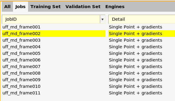
Here, you see that all jobs are of type “Single Point + gradients”. This is the only type of job that can be used during the training. The job collection can also contain other types of jobs, but they will then not be used during the training but will simply be run after the training has finished.

Tip

When importing training data into ParAMS:

• Use the “add trajectory singlepoints” importer to import data from trajectories

• Use the “add pesscan singlepoints” importer to import data from PES scans

• If you use the “add single job” importer, make sure that “Task (for new job)” is set to singlepoint !

Switch to the Training set panel

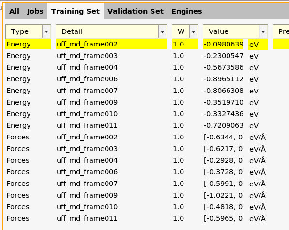
Here, you can see energies and forces for the training set.

Switch to the Validation set panel

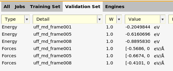
Here, you can see energies and forces for the validation set.

For task Machine Learning, you should always have at least one entry in the validation set.

Note

The energy and forces for a given job must belong to the same data set.

Example: Both the energy and forces for uff_md_frame001 are in the validation set. It is not allowed to split these so that for example the energy is in the training set and the forces in the validation set.

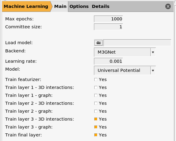
4.1.3. Machine learning basic settings

The bottom left panel shows the machine learning settings.

• Max epochs is the maximum number of epochs for the training.

• Committee size specifies how many independent ML models to train. The average of all models is taken as the final predicted energy/forces. Setting this to a number larger than 1 will significantly increase the computational cost and memory requirements, but will let you get a measure for the uncertainty of the predicted values.

• Load model lets you load a previous model from a ParAMS results directory. In this way, you can continue training from previous results, either for more epochs or with extra training data.

• Backend: What type of machine learning model to use. Here we use M3GNet. Note that you must first separately install M3GNet from the AMS package manager (SCM → Packages).

• Learning rate: The learning rate.

For the M3GNet backend, you can select two different Models:

• Custom: this trains a new neural network completely from scratch. You can decide the architecture for this neural network, for example the number of neurons per layer and the number of convolution blocks. Note that you will typically require quite a lot of training data to train a good model using Custom.

• UniversalPotential: this starts the training from the M3GNet-UP-2022 universal potential. This typically makes training much faster. You can choose which layers to retrain, but not change any other parameters.

Set Max epochs to 150

Set Model to Universal Potential.

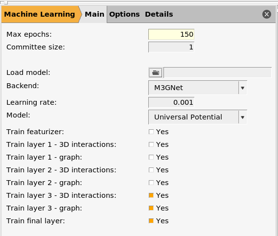
4.1.4. Other machine learning settings

In the bottom left panel, switch to the Options → Loss Function panel

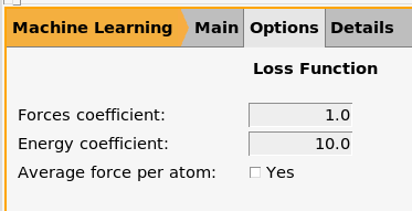
For task Machine Learning, the weights of the different training set entries can be set both

• in the “W” column in the top right table (on the training set and validation set panels), and

• on the Options → Loss function settings panel.

The W column lets you set different weights for different individual entries. On the Options → Loss function panel, you can instead set the relative weights for energy and forces.

If you find that the energy is not trained accurately enough, you may consider increasing the Energy coefficient on the Options → Loss function panel.

In the bottom left panel, switch to the Options → Targets panel

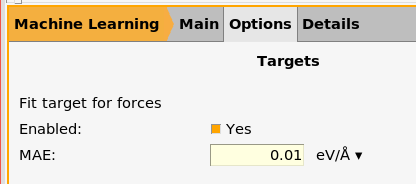
This panel lets you set a target value for the MAE on the forces. This means that if the MAE is smaller than this threshold for both the training and validation, the training stops. This can help to

• prevent overfitting, and

• stop the training when the model has acceptable accuracy in order to not keep on training when the model is already good enough

4.1.5. Run the M3GNet training

File → Save As, and save the job with the name m3gnet_tutorial.params

File → Run (or run the job from AMSjobs)

Wait for the job to finish. It may take a few minutes.

4.1.6. View the M3GNet training results

In the bottom right panel, select the Graphs tab

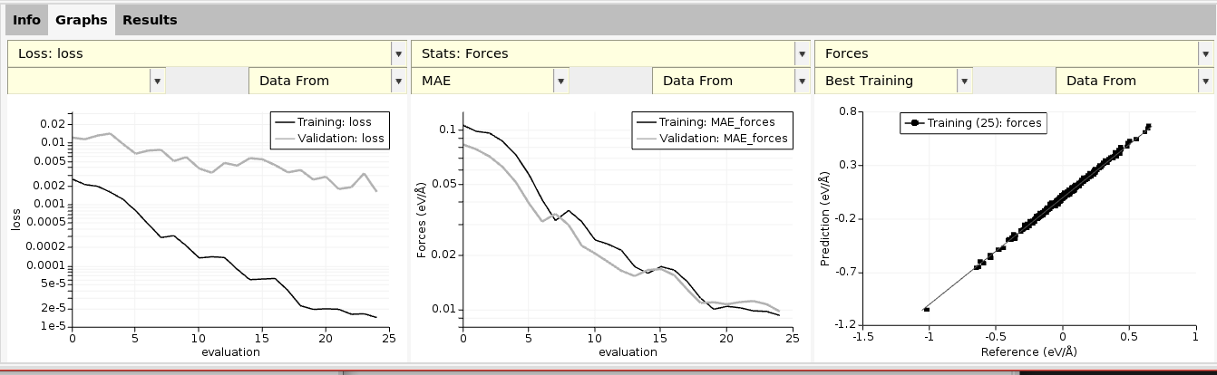
Here, you can see graphs for loss function and stats vs. epoch.

You may find that the training ended in fewer than the 150 maximum epochs. This is because both the training and validation MAE on the forces became smaller than 0.01 eV/Å (the Target value that was specified).

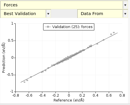
At the end of the training, you also get a scatter plot with predicted vs. reference forces and energies. You can switch between Best training and Best validation to see the training and validation performance.

Note

For Task MachineLearning, the scatter plot only appears when the training has finished.

4.1.7. Use the retrained model for production calculations

In the bottom right panel, select the Results tab

In the drop-down, select Validation best: engine (or Training best: engine)

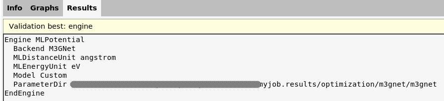
This shows the contents of part of the AMS text input file you would need to provide to use the retrained model in a production calculation. In particular, it shows you the ParameterDir containing the trained parameters.

Tip

Copy the ParameterDir directory to some place that is easier to access, in case you want to reuse it many times.

There are two ways to import these engine settings into AMSinput:

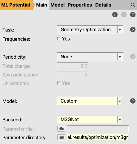
4.1.7.1. Method 1: Open optimized engine in AMSinput

File → Open Optimized Engine in AMSinput → Best validation

This opens a new AMSinput window with the MLpotential engine selected. This gives you a warning to double-check the input. It should switch automatically to the MLpotential engine with Model Custom. If you click the next to Custom, you will additionally see the path to the ParameterDir and the units used.

4.1.7.2. Method 2: Copy-paste into AMSinput

Select the entire Engine MLPotential … EndEngine block

Edit → Copy

SCM → New Input

In the newly opened AMSinput window: Edit → Paste

This gives you a warning to double-check the input. It should switch automatically to the MLpotential engine with Model Custom. If you click the next to Custom, you will additionally see the path to the ParameterDir and the units used.