1. General
1.1. What is ParAMS?
ParAMS is a module in the Amsterdam Modeling Suite for training/reparameterizing
ReaxFF,
DFTB (GFN1-xTB), and
Machine Learning potentials
There is both a graphical user interface (GUI) and a Python library.
To get started, see the Getting Started: Lennard-Jones tutorial.
Selected features:
Import reference data from AMS, VASP, Quantum ESPRESSO, Gaussian, or experiment
Use a validation set to prevent overfitting
Submit jobs to remote machines using the GUI
Results updated on the fly in the GUI with many diagrams
For ReaxFF and DFTB (Task: Optimization):
Fit any number of properties: reaction energies, forces, bond lengths, angles, cell parameters, stress tensors, charges, …
Use single points, geometry optimizations, or PES scans during the parametrization
Set custom weights for different training set entries
Choose which parameters to optimize, and set allowed ranges for them
Optimize with CMA-ES or Nelder-Mead
Intuitive output files for creating correlation plots, energy-volume curves, and more
For ML Potentials (Task: MachineLearning):
Fit energies and forces for single-point calculations
Use transfer learning to retrain the M3GNet universal potential to your specific chemistry
Train committee models that provide uncertainty estimates
Intuitive output files for monitoring the optimization, creating correlation plots, and more
Use ParAMS in the Simple Active Learning workflow to train your model on the fly during MD simulations
See also
1.2. What’s new in ParAMS 2025?
New simpler way to use Task SinglePoint with a single engine for benchmarks by specifying engine input directly in the params.in file (thus avoiding the need to set up a parameter interface and engine collection).
Importing molecular dynamics simulations with changing number of atoms such as the Molecule Gun as single points is now supported.
1.3. What’s new in ParAMS 2024?
Fit machine learning models with Task MachineLearning (tutorials, documentation).
ParAMS can now be used during active learning for machine learning potentials.
Split a Data Set using split_by_jobid to make sure that e.g. energies and forces extracted from the same job end up in the same subset.
1.4. What’s new in ParAMS 2023?
Run multiple optimizers in parallel (tutorial)
Automatically or manually turn off and restart optimizers not performing well
Run a “single point” saving all jobs to disk (tutorial, docs)
The input file is now called
params.inand follows the same syntax as other AMS programs. You can easily convert the oldparams.conf.pyto aparams.infile (done automatically by the GUI).Import results (energy and forces) from Gaussian .out files
New parameter interface: No parameters (empty interface), can be used together with
Task SinglePointto run benchmarks with engine settings that are completely defined in the engine collection (thus any AMS engine settings can be used, not just the engines that can be parametrized).New parameter interface: ASE Parameters, can be used to parametrize a custom ASE calculator. Requires an MLPotential license.
The
pesextractor can now be used with the argumentrelative_to="previous"to fit the derivative of a PESScan energy curve.New extractors: band gap, band structure. Note: Make sure to set UsePipe No when using these!
The GUI can now apply recommended ReaxFF parameter constraints for some parameters. Select the parameters and choose Parameters → Apply Recommended Constraints.
Technically, ParAMS now uses GloMPO (globally managed parallel optimizers) to run the parameter optimization.
Changes potentially breaking old ParAMS scripts:
Callbacks no longer exist. You can achieve the same functionality using other input options.
The
params.conf.pyno longer exists. The input format has changed. The input file is now called params.in.
Other changes:
The Settings panel in the GUI has been fully reworked and is now much easier to use. It expands when you click on it.
1.5. What’s new in ParAMS 2022?
The AMS2022.1 release is the first version to include a GUI for ParAMS. The ParAMS GUI replaces the previous AMStrain module for ReaxFF parametrization.
Other changes:
The Results Importer class provides a shortcut for reading structures, reference results, and engine settings from finished reference job.
The Logger output structure has been changed, with many new useful output files
Job-dependent engine settings using the JCEntry.extra_engine attribute
Parameter interfaces can be stored in text .yaml format
Exact restarts with the CMA-ES optimizer
Support for reading in VASP OUTCAR files and Quantum ESPRESSO .out files
Weights schemes for setting individual datapoint weights for array reference values (for example, to weight large force components less than small force components)
Initialize an empty ReaxFFParameters using
ReaxFFParameters(None)Copy blocks of parameters from ReaxFF force field files
New class names: ReaxParams → ReaxFFParameters, xTBParams → GFN1xTBParameters
New variable names (e.g. in the Optimization class constructor and in params.conf.py): jobcollection → job_collection, enginecollection → engine_collection, dataset → data_set, interface → parameter_interface
Scalar weights for array reference values are interpreted as the sum of weights: weight = 1 for an array of length 3 gives each point a weight of 0.3333 (before, the scalar value was broadcasted so the total weight would be 3).
Faster reading of Job Collections
Support for gzip-compressed job collections and training sets
All extractors have explicit default units and sigma values
Distance, angle, and dihedral extractors use the minimum image convention under periodic boundary conditions by default
The params main script supports validation sets
ParAMS requires a valid license
1.6. Theory of Parameter Fitting: A Lennard-Jones Example
See also
Tutorial: Getting Started: Lennard-Jones
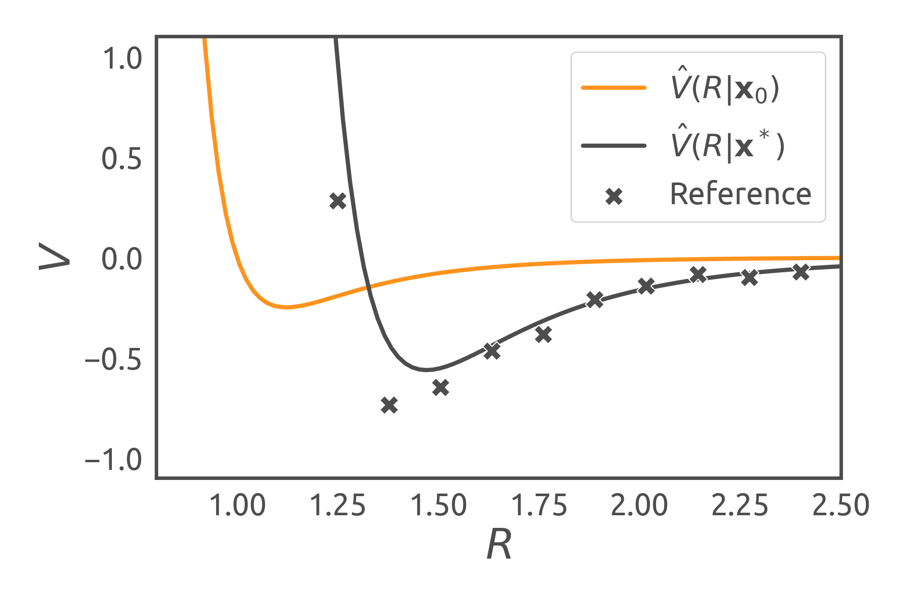
Assuming we are interested in calculating the potential energy \({V}(R)\) between two Argon atoms, one suitable model for this task is the Lennard-Jones Potential (LJ), which is given by
where \(\hat{V}\) is the (predicted) potential energy as a function of the interatomic distance \(R\) and a parameter vector \(\boldsymbol{x}=({x_ 1}, {x_2})^\mathrm{T}\) that modifies the shape of the potential.
If reference data \(\boldsymbol{y} = \{(R_i,V_i)\}\) is available for this problem (either from an experiment or another model), we can measure the quality of the LJ model by a loss function (also called objective or cost function) \(L\), which is a metric operating on the residuals vector \(\boldsymbol{y} - \boldsymbol{\hat{y}} = \{V_i - \hat{V}_i\}\). One example for such a metric is the mean absolute error (MAE):
For a case when the LJ model perfectly represents the experimental data, \(\boldsymbol{y} = \boldsymbol{\hat{y}}\), and \(L=0\). In contrast, a larger loss function value represents a mismatch between the predicted and reference values. In such cases the parametric model’s parameters can be fitted, assuming the reference set of systems and energies does not change during the optimization process. We introduce an optimizer which produces an optimized set of parameters \(\boldsymbol{x}^*\) from an initial point \(\boldsymbol{x}_0\) by minimizing \(L\):
We visualize the influence of two different parameter sets for the Lennard-Jones potential in the figure below: While the initial model parameters (orange curve) might not represent experimental data (discrete marks) very well, an optimization of the parameters with respect to the reference data can provide a viable solution (grey curve).
1.7. General Application
In a more generalized description of the package, ParAMS allows its users to fit a variety of parametric (empirical) models that are part of the Amsterdam Modeling Suite. By design, any physicochemical property \(P\) that can be extracted from one AMS computation (or constructed from multiple), can be fitted with a number of different optimizers. A minimal setup does not require much additional user input, making basic workflows easy and accessible to set up.
At the same time, ParAMS offers a variety of additional features for customizing the workflow such as automated and manual definition of the search space, relevant parameter subsets, or support for validation sets, to name a few, resulting in a package that is highly flexible when it comes to advanced user requirements.
Integration with AMS guarantees that the same APIs are supported regardless of the application, making workflows highly reusable and storage of relevant reference data in the human-readable YAML format ensures transparency and reproducibility.