2.2. Getting Started: Lennard-Jones
This example illustrates how to fit a Lennard-Jones potential. The systems are snapshots from a liquid Ar MD simulation. The forces and energies (the reference data) were calculated with dispersion-corrected DFTB.
Note
In this tutorial the training data has already been prepared. See how it was generated further down.
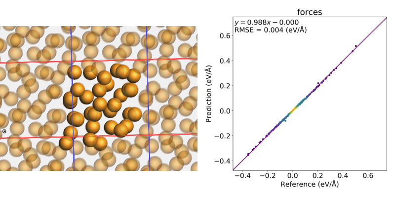
Fig. 2.1 Left: One of the systems in the job collection. Right: predicted (with parametrized Lennard-Jones) forces compared to reference (dispersion-corrected DFTB) forces.
Tip
Each step of the tutorial covers
How to use the ParAMS graphical user interface
How to run or view results from the command-line
2.2.1. Lennard-Jones Parameters, Engine, and Interface
The Lennard-Jones potential has the form
where \(\epsilon\) and \(\sigma\) are parameters. The Lennard-Jones engine in AMS has the two parameters Eps (\(\epsilon\)) and RMin (distance at which the potential reaches a minimum), where \(\text{Rmin} = 2^{1/6}\sigma\).
In ParAMS, those two parameters can be optimized with the Lennard-Jones
parameter interface, which is used in this example. The
parameters then have the names eps and rmin (lowercase).
2.2.2. Files
Download LJ_Ar_example.zip and unzip the file, or make a copy of the directory $AMSHOME/scripting/scm/params/examples/LJ_Ar.
The directory contains four files (parameter_interface.yaml, job_collection.yaml, training_set.yaml, and params.in) that you can view and change in the ParAMS graphical user interface (GUI). If you prefer, you can also open them in a text editor.
LJ_Ar
├── job_collection.yaml
├── parameter_interface.yaml
├── params.in
├── lennardjones.py
├── README.txt
└── training_set.yaml
2.2.3. Workflows
ParAMS 2023 provides three workflows:
GUI: Recommended main interface allowing you to easily setup tasks, visualize results, and submit local or remote jobs.
Command-line: Console interface for systems without GUI support (e.g. submitting jobs on a cluster).
Scripting: Python/PLAMS interface to ParAMS allowing you to integrate it into data workflows and easily setup multiple configurations. Use the
$AMSBIN/amspythonprogram to execute python scripts.
All of them are based on the new params.in input file which follows the AMS-style input language (see Input file: params.in for more details).
In this tutorial we will demonstrate how to complete the optimization in all three ways.
The python script (lennardjones.py) has already been prepared for you, and we will be referring to it in the Scripting tabs throughout the tutorial.
2.2.4. ParAMS input
2.2.4.1. Parameter interface (parameter_interface.yaml)
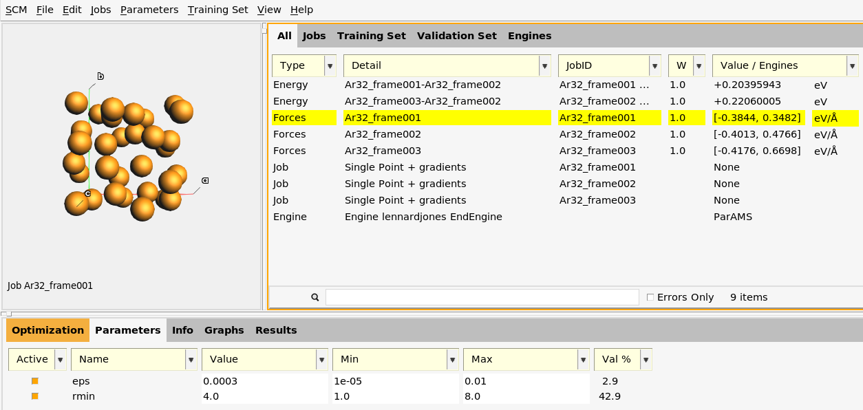
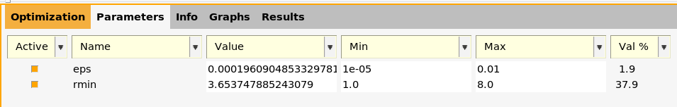
The parameters are shown on the Parameters tab.
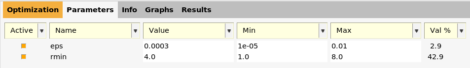
All the parameters in a
parameter interface have names. For Lennard-Jones, there are only two
parameters: eps and rmin.
Every parameter has a value and an allowed range of values.
Above, the value for eps is shown to be 0.0003, and the allowed
range to between 1e-5 and 0.01. This means that the eps
variable will only be varied between \(10^{-5}\) and
\(10^{-2}\) during the parametrization.
Similarly, the initial value for rmin is set to 4.0, and the allowed range is between 1.0 and 8.0.
Note
You can edit the parameter values and the allowed ranges directly in the table.
The Active attributes of the parameter set are checked, meaning that they will be optimized. To skip optimizing a parameter, untick the Active checkbox.
The Val % column indicates how close to the Min or Max that the
current value is. It is calculated as 100*(value-min)/(max-min). For
example, for rmin, it is 100*(4.0-1.0)/(8.0-1.0) = 42.9. It has
no effect on the parametrization; it only lets you quickly see if the
value is close to the Min or Max.
The parameter_interface.yaml file is a Parameter Interface of type LennardJonesParameters. It contains the following:
 1---
 2dtype: LennardJonesParameters
 3settings:
 4  input:
 5    lennardjones: {}
 6version: '2022.101'
 7---
 8name: eps
 9value: 0.0003
10range:
11- 1.0e-05
12- 0.01
13is_active: true
14atoms: []
15---
16name: rmin
17value: 4.0
18range:
19- 1.0
20- 8.0
21is_active: true
22atoms: []
23...
All the parameters in a
parameter interface have names. For Lennard-Jones, there are only two
parameters: eps and rmin.
Every parameter needs an initial value and an allowed range of values.
Above, the initial value for eps is set to 0.0003, and the allowed range to between 1e-5 and 0.01.
This means that the eps variable will only be varied between \(10^{-5}\) and \(10^{-2}\)
during the parametrization.
Similarly, the initial value for rmin is set to 4.0, and the allowed range is between 1.0 and 8.0.
The is_active attribute of the parameters is set to True, meaning that they will be optimized.
For details about the header of the file (lines 2-6), see the parameter interface documentation.
To create or modify a parameter_interface.yaml file in Python, you would do something like the following:
from scm.params import *

lj = LennardJonesParameters.yaml_load('parameter_interface.yaml') # load existing
lj['eps'].value = 0.0003
lj['eps'].is_active = True
lj['eps'].range = (1e-5, 1e-2)
lj['rmin'].value = 4.0
lj.yaml_store('new_parameter_interface.yaml') # store in new file
For details, see the Parameter Interfaces, Lennard-Jones, ReaxFF, or GFN1-xTB documentation.
2.2.4.2. Job Collection (job_collection.yaml)
The Jobs panel contains three entries. They have the JobIDs Ar32_frame001, Ar32_frame002, and Ar32_frame003.
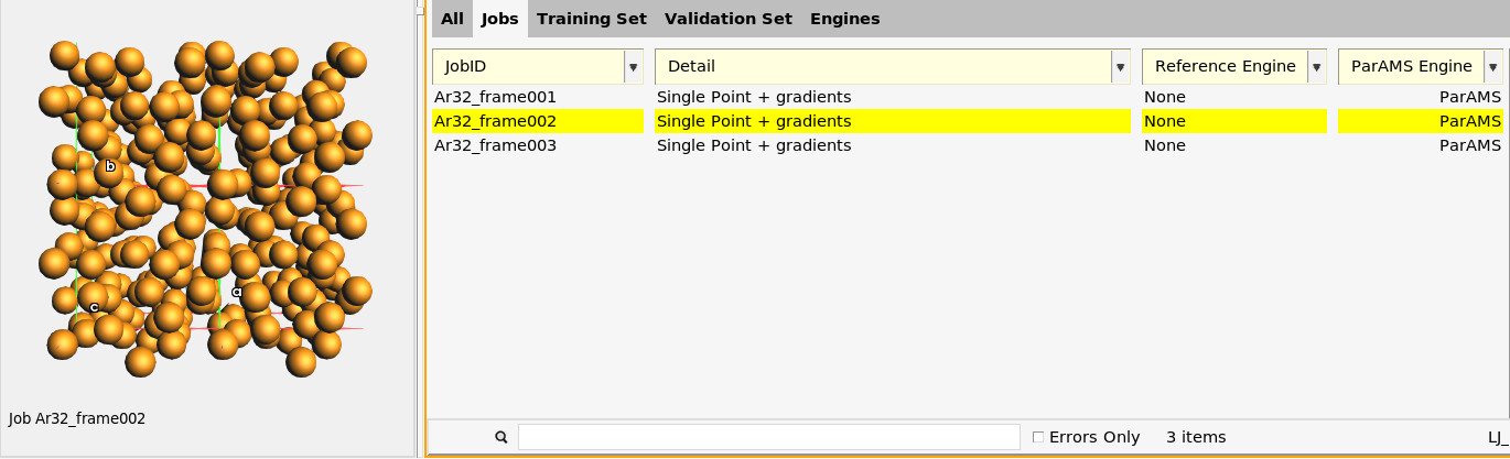
The Jobs panel has four columns:
JobID: The name of the job. You can rename a job directly in the table by first selecting the row, and then clicking on the job id.
Detail: Some information about the job. SinglePoint + gradients means that a single point calculation on the structure is performed, also calculating the gradients (forces). Double-click in the Detail column for a job to see and edit the details. You can also toggle the Info panel in the bottom half.
Reference Engine: This column can contain details about the reference calculation, and is described more in the tutorials Import training data (GUI) and Generate reference values.
ParAMS Engine: This column can contain details about job-specific engine settings. It is described in the tutorial GFN1-xTB: Lithium fluoride
The job_collection.yaml file is a Job Collection. It contains entries like these:
 1---
 2dtype: JobCollection
 3version: '2022.101'
 4---
 5ID: 'Ar32_frame001'
 6ReferenceEngineID: None
 7AMSInput: |
 8   properties
 9     gradients Yes
10   End
11   system
12     Atoms
13                Ar       5.1883477539      -0.4887475488       7.9660568076
14                Ar       5.7991822399       0.4024595652       2.5103286966
15                Ar       6.1338265157       5.5335946219       7.0874208384
16                Ar       4.6137188191       5.9644505949       3.0942810122
17                Ar       8.4186778390       7.6292969115       8.0729664423
18                Ar       8.3937816110       8.6402371806       2.6057806799
19                Ar       7.5320205143       1.7666481606       7.7525889818
20                Ar       8.5630139885       2.0472039529       2.6380554086
21                Ar       2.6892353632       7.8435284207       7.7883054306
22                Ar       2.4061636915       7.5716025415       2.4535180075
23                Ar       2.2485171283       2.9764130946       7.8589298904
24                Ar       3.0711058946       1.8500587164       2.5620921469
25                Ar       7.6655637500      -0.4865893003       0.0018797080
26                Ar       7.7550067215      -0.0222821825       4.8528637785
27                Ar       7.7157262425       4.6625079517      -0.3861722152
28                Ar       7.7434900996       5.2619590353       4.2602386226
29                Ar       3.4302237084      -0.2708640738       0.6280466620
30                Ar       2.8648051689       0.6106220610       6.1208342905
31                Ar       3.2529823775       5.7151788324      -0.2024448179
32                Ar       2.0046357208       4.9353027402       5.4968740217
33                Ar       0.9326855213       8.0600564695      -0.3181225099
34                Ar      -0.5654205469       8.5703446434       5.8930973456
35                Ar      -0.9561293133       2.1098403312      -0.0052667919
36                Ar      -0.8081417664       3.2747992855       5.5295389610
37                Ar       5.5571960244       7.5645919074       0.1312355350
38                Ar       4.4530832384       7.6170633330       5.4810860433
39                Ar       5.1235367625       2.7983577675      -0.3161069611
40                Ar       5.2048439076       2.9885672135       4.5193274119
41                Ar      -0.2535891591       0.0134355189       8.3061692970
42                Ar       0.5614183785      -0.1927751317       3.2355155467
43                Ar      -0.0234943080       5.0313863031       8.0451075074
44                Ar      -0.4760138873       6.2617510830       2.5759742219
45     End
46     Lattice
47           10.5200000000     0.0000000000     0.0000000000
48            0.0000000000    10.5200000000     0.0000000000
49            0.0000000000     0.0000000000    10.5200000000
50     End
51   End
52   task singlepoint
Each job collection entry has an ID (above Ar32_frame001) and some
input to AMS, in particular the structure (atomic species, coordinates, and
lattice). Each entry in the job collection constitutes a job that is
run for every iteration during the parametrization.
What to extract from the jobs is defined in Training Set (training_set.yaml).
The class JobCollection can be used
to create or modify job_collection.yaml files.
from scm.params import *

jc = JobCollection('job_collection.yaml') # load existing
for job_id in jc:
    print(job_id)
    print(jc[job_id])
jc.store('new_job_collection.yaml') # store in new file
To create a job collection, we recommend to use a Results Importer. See Appendix: Creation of the input files or Import Training Data with ResultsImporter.
2.2.4.3. Training Set (training_set.yaml)
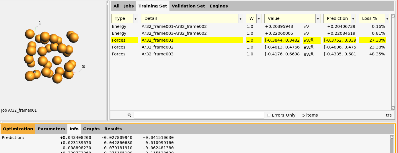
The Training Set panel contains five entries: two of type Energy and three of type Forces.
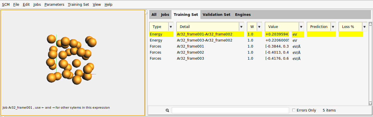
The first Energy entry has the Detail Ar32_frame001-Ar32_frame002.
This means that for every iteration during the parametrization, the
current Lennard-Jones parameters will be used to calculate
the energy of the job Ar32_frame001 minus the energy of the job
Ar32_frame002. The number should ideally be as close as possible to
the reference value, which is given as 0.204 eV in the Value
column. The greater the deviation from the reference value, the more
this entry will contribute to the loss function.
Double-click in the Detail column for the first entry to see some more details.
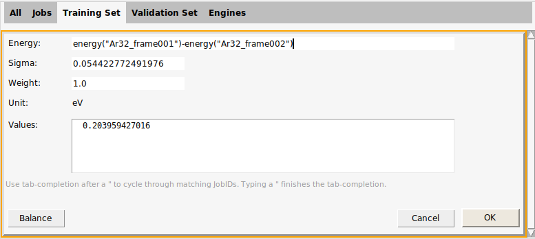
This brings up a dialog where you can change
What is calculated (the Energy text box). For example,
energy("Ar32_frame001")extracts the energy of the Ar32_frame001 job. You can combine an arbitrary number of such energies with normal arithmetic operations (+, -, /, *). For details, see the Import training data (GUI) tutorial.Sigma: A number signifying an “acceptable prediction error”. Here, it is given as 0.0544 eV, which is the default value for energies. A smaller sigma will make the training set entry more important (contribute more to the loss function). For beginning ParAMS users, we do not recommend to modify Sigma, but instead to modify the Weight.
Weight: A number signifying how important the training set entry is. A larger weight will make the training set entry more important (contribute more to the loss function). The default weight is 1.0.
Note
The Sigma for a training set entry is not the σ that appears in the Lennard-Jones equation. For more information about Sigma and Weight, see Sigma vs. weight: What is the difference?.
Unit: The unit that Sigma and the reference value are expressed in. Here, it is set to eV. See how to set preferred units.
Value: The reference value (expressed in the unit above).
Click OK. This brings you back to the Training Set panel.
The W column contains the Weight of the training set entry. You can edit it directly in the table.
The Value column contains the reference value.
The Prediction column contains the predicted value (for the “best” parameter set) for running or finished parametrizations. It is now empty.
The Loss % column contains the how much an entry contributes to the loss function (in percent) for running or finished parametrizations. It is now empty.
Many different quantities can be extracted from a job.
The third entry is of type Forces for the job Ar32_frame001.
The reference data are the atomic forces (32 × 3 force components) from the job
Ar32_frame001. The Value column gives a summary: [-0.3844, 0.3482] (32×3), meaning
that the most negative force component is -0.3844 eV/Å, and the most positive force component
is +0.3482 eV/Å.
To see all force components, either double-click in the Details column or switch to the Info panel at the bottom.
The training_set.yaml file is a Data Set.
It contains entries like these:
 1---
 2dtype: DataSet
 3version: '2022.101'
 4---
 5Expression: energy('Ar32_frame001')-energy('Ar32_frame002')
 6Weight: 1.0
 7Sigma: 0.054422772491975996
 8ReferenceValue: 0.20395942701637979
 9Unit: eV, 27.211386245988
10---
11Expression: energy('Ar32_frame003')-energy('Ar32_frame002')
12Weight: 1.0
13Sigma: 0.054422772491975996
14ReferenceValue: 0.22060005303998803
15Unit: eV, 27.211386245988
16---
17Expression: forces('Ar32_frame001')
18Weight: 1.0
19Sigma: 0.15426620242897765
20ReferenceValue: |
21   array([[ 0.04268692, -0.02783233,  0.04128417],
22          [ 0.02713834, -0.04221017, -0.01054571],
23          [-0.00459236, -0.07684888,  0.06155902],
24          [ 0.34815492, -0.38436427, -0.12292068],
25          [-0.20951048, -0.09704763,  0.30684271],
26          [-0.12165704,  0.02841069, -0.03455513],
27          [-0.01065992,  0.04707562, -0.00797079],
28          [-0.09806036,  0.06893426,  0.29291125],
29          [-0.08117544,  0.00197622,  0.05092921],
30          [-0.26343319,  0.26285542, -0.02473382],
31          [ 0.06144345, -0.01781664,  0.17121465],
32          [-0.16915463,  0.24386843,  0.13151148],
33          [-0.01651514,  0.03927323, -0.12482729],
34          [-0.05972447,  0.09258089,  0.23253252],
35          [ 0.00554623,  0.0802643 ,  0.00565681],
36          [-0.14037904,  0.02969844,  0.01099823],
37          [-0.03492464, -0.20821058, -0.25464835],
38          [-0.01710259, -0.10689741, -0.13469458],
39          [-0.12217555, -0.15624485, -0.02885505],
40          [ 0.04492738,  0.08596881, -0.11475184],
41          [-0.15375715,  0.02301999,  0.09411744],
42          [ 0.26855338,  0.0068943 , -0.31912743],
43          [ 0.19519975,  0.05424052, -0.29197409],
44          [ 0.03589698, -0.11822402,  0.00851084],
45          [ 0.12697447,  0.08277883,  0.01592771],
46          [ 0.10473145,  0.18847622, -0.03627933],
47          [-0.03520977, -0.03814586,  0.0023055 ],
48          [ 0.05408552,  0.02290898,  0.08376102],
49          [ 0.06093887,  0.00964534, -0.01148707],
50          [ 0.02291482,  0.01746282,  0.00389746],
51          [-0.07331299,  0.09730838,  0.08506009],
52          [ 0.21215231, -0.20979905, -0.08164896]])
53Unit: eV/angstrom, 51.422067476325886
54---
The first entry has the Expression
Expression: energy('Ar32_frame001')-energy('Ar32_frame002')
which means that for every iteration during the parametrization, the current Lennard-Jones parameters will be used to calculate the energy of the job Ar32_frame001 minus the energy of the job Ar32_frame002. The number should ideally be as close as possible to the ReferenceValue, which above is given as 0.204 eV. The greater the deviation from the reference value, the more this entry will contribute to the loss function.
The Weight and Sigma also affect how much the entry contributes to the loss function. For details, see Data Set and Sigma vs. weight: What is the difference?.
Note
The Sigma in training_set.yaml is not the \(\sigma\) that appears in the Lennard-Jones equation.
Reference data can be expressed in any Unit. The Unit for the first expression
is given as eV, 27.21138. The number specifies a conversion factor from the
default unit Ha. If no Unit is given, the data must
be given in the default unit.
Many different quantities can be extracted from a job. The third entry (starting on line 17) has the Expression
Expression: forces('Ar32_frame001')
which extracts the atomic forces (32 × 3 force components) from the job
Ar32_frame001. The reference value for the force components are given as a matrix
in eV/angstrom (as specified by the Unit).
The class DataSet can be used
to create or modify training_set.yaml files.
from scm.params import *

data_set = DataSet('training_set.yaml') # load existing
for entry in data_set:
    print(entry.expression)
data_set.store('new_training_set.yaml') # write to new file
To create a training set, we recommend to use a Results Importer. See Appendix: Creation of the input files or Import Training Data with ResultsImporter.
2.2.4.4. ParAMS settings (params.in)
Click  to open the input panel.
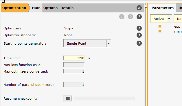
The Main panel on the flyout contains all of the most important options.
You can see that the two options in the params.in input file appear here:
Optimizer: Scipy
Time limit: 120 s
Optimizer: This option selects the optimizer which should be used on the problem. For simple optimization problems like Lennard-Jones, the Nelder-Mead method from SciPy can be used. For more complicated problems, like ReaxFF optimization, a more advanced optimizer like the CMA-ES is recommended (see for example the ReaxFF (basic): H₂O bond scan tutorial).
Time limit: This option specifies the time limit of the optimization. If the parametrization takes longer than two minutes (120 seconds), it will stop. If you remove the option (by clearing the contents of the field) then there is no time limit.
Max Optimizers Converged: This is an alternative termination option. It specifies that we would like to stop the optimization as soon as the optimizer is done. Since we have two Exit Conditions, the optimization will stop when either condition is met.
Note
The Max Optimizers Converged condition is required in AMS2023 or later. In AMS2022 you could only run a single optimizer at a time. Thus, the optimization would always end when the optimizer ended. In AMS2023 you can now run multiple optimizers in parallel or sequentially. Therefore, you need to specify exactly when you would like to exit. Without this condition, if the optimizer stopped before the two minute time limit, ParAMS would start a new optimizer.
There are also many other options. For this tutorial we will remain with the basics.
The params.in file uses the AMS input-syntax and contains
 1Task Optimization
 2
 3JobCollection job_collection.yaml
 4
 5ParameterInterface parameter_interface.yaml
 6
 7DataSet
 8  Name training_set
 9  Path training_set.yaml
10End
11
12ParallelLevels
13    Optimizations 1
14    ParameterVectors 1
15    Jobs 1
16    Processes 1
17End
18
19Optimizer
20  Type Scipy
21  Scipy
22    Algorithm Nelder-Mead
23  End
24End
25
26ExitCondition
27  Type TimeLimit
28  TimeLimit 2600
29End
30
31ExitCondition
32    Type MaxOptimizersConverged
33    MaxOptimizersConverged 1
34End
Task: This key specifies the type of job we would like to carry out. In this case, an optimization, but ParAMS also allows you to also specify other tasks (see Input file: params.in).
JobCollection: This key is a path to the job_collection.yaml file.
ParameterInterface: This key is a path to the parameter_interface.yaml file.
DataSet: This block specifies all the options related to a data set and how it should be evaluated. Multiple datasets are allowed, each must have a unique Name and a Path to their corresponding YAML file.
ParallelLevels: This block specifies how to run in parallel. Here, we choose to run in serial (on 1 core only).
Optimizer: This block specifies the Type of optimizer to use during the parameterization, as well as its configuration settings. For simple optimization problems like Lennard-Jones, the Nelder-Mead method from SciPy can be used. For more complicated problems, like ReaxFF optimization, a more advanced optimizer like the CMA-ES is recommended (see for example the ReaxFF (basic): H₂O bond scan tutorial).
ExitCondition: These are blocks specifying under what conditions that optimization should stop. Multiple conditions may be used at the same time. One block specifies the time limit of the optimization. If the parametrization takes longer than two minutes (120 seconds), it will stop. If you remove this block then there is no time limit. The other block specifies that we would like the optimization to stop once one optimizer has converged (instead of starting a second optimizer).
Note
The MaxOptimizersConverged condition is required in AMS2023. In AMS2022 you could only run a single optimizer at a time. Thus, the optimization would always end when the optimizer ended. In AMS2023 you can now run multiple optimizers in parallel or sequentially. Therefore, you need to specify exactly when you would like to exit. Without this condition, if the optimizer stopped before the two minute time limit, ParAMS would start a new optimizer.
There are also many other options. For this tutorial we will remain with the basics.
To set up the job settings in python, see the setup_job() function in lennardjones.py.
For a detailed explanation, see the ParAMS Python examples.
def setup_job():
    """Returns: a ParAMSJob"""
    job = ParAMSJob(name="lennardjones")

    job.settings.input.Task = "Optimization"

    job.parameter_interface = "parameter_interface.yaml"
    job.job_collection = "job_collection.yaml"
    job.training_set = "training_set.yaml"

    job.settings.input.ParallelLevels.Optimizations = 1
    job.settings.input.ParallelLevels.ParameterVectors = 1
    job.settings.input.ParallelLevels.Jobs = 1
    job.settings.input.ParallelLevels.Processes = 1

    job.add_optimizer("Scipy", {"Algorithm": "Nelder-Mead"})

    job.add_exit_condition("TimeLimit", 120)
    job.add_exit_condition("MaxOptimizersConverged", 1)

    return job
Tip
In lennardjones.py we have setup the job manually for tutorial purposes.
However, we could have loaded the existing params.in file for a quicker setup:
job = ParAMSJob.from_inputfile(path='params.in', name='lennardjones')
2.2.5. Run the example
Save the project with a new name. If the name does not end with .params, then .params will be added to the name.
lennardjones.params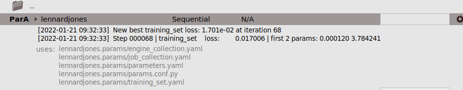
Tip
Using AMSjobs you can also submit ParAMS jobs to remote queues (compute clusters).
Start a terminal window as follows:
Windows: In AMSjobs, select Help → Command-line, type
bashand hit Enter.MacOS: In AMSjobs, select Help → Terminal.
Linux : Open a terminal and
source /path/to/ams/amsbashrc.sh
In the terminal, go to the LJ_Ar directory, and run the ParAMS Main Script:
"$AMSBIN/params"
which gives beginning output similar to this:
[16.03|16:24:30] Checking project for consistency ...
[16.03|16:24:30] No issues found in data sets.
[16.03|16:24:30] No issues found in parameter interface.
[16.03|16:24:30] Exporting settings and initial data:
[16.03|16:24:30] Export done!
[16.03|16:24:30] Starting parameter optimization. Dim = 2
PLAMS working folder: /tmp/plams_workdir.002
[16.03|16:24:30] Initial loss: 5.722e+02
[16.03|16:24:30] Initializing Manager ...
[16.03|16:24:30] Manager will not force-stop optimizers.
[16.03|16:24:30] Checkpointing requested but this is not supported by Scipy optimizers. Checkpoints will not behave as expected.
[16.03|16:24:30] Initialization Done
[16.03|16:24:30] System Info:
    Cores Available:..........20
    Core IDs:.................[0, 1, 2, 3, 4, 5, 6, 7, 8, 9, 10, 11, 12, 13, 14, 15, 16, 17, 18, 19]
    Memory Available:.........24.11GB
    Hostname:.................scmlaptop13
    Current Dir:............../home/spiering/Desktop/release2023/tutorials/ParametrizationParAMS/GettingStartedLennardJones/Step6_RunExample_GUI/tmp.spiering.51577.0.noindex
    Output Dir:.............../home/spiering/Desktop/release2023/tutorials/ParametrizationParAMS/GettingStartedLennardJones/Step6_RunExample_GUI/RunExample.results/optimization
    Username:.................spiering
[16.03|16:24:30] Starting GloMPO Optimization Routine
[16.03|16:24:30] Setting up optimizer 1 of type Scipy
[16.03|16:24:30] Starting Optimizer: 1
[16.03|16:24:30] Status: 1 optimizers alive, 1/1 slots filled, 0 function evaluations, f_best = None.
[16.03|16:24:30] New best training_set loss: 5.722e+02 at iteration 1
[16.03|16:24:30] Step 000001 training_set    loss:      572.188673 | first 2 params: 0.000300 4.000000
[16.03|16:24:30] New best training_set loss: 5.062e-01 at iteration 2
[16.03|16:24:30] Step 000002 training_set    loss:        0.506209 | first 2 params: 6.47500000e-05 4.000000
[16.03|16:24:30] New best training_set loss: 7.795e-02 at iteration 4
[16.03|16:24:30] Step 000004 training_set    loss:        0.077947 | first 2 params: 6.47500000e-05 3.975000
[16.03|16:24:48] Step 000185 training_set    loss:        0.002514 | first 2 params: 0.000196 3.653746
[16.03|16:24:48] New best training_set loss: 2.514e-03 at iteration 188
[16.03|16:24:48] Step 000188 training_set    loss:        0.002514 | first 2 params: 0.000196 3.653748
[16.03|16:24:49] Signal 0 from 1.
[16.03|16:24:49] Exit triggered
[16.03|16:24:49] Exiting manager loop
[16.03|16:24:49] Exit conditions met:
                         TimeLimit(session_max=120.0, overall_max=None) = False |
                         MaxOptimizersConverged(nconv=1) = True
[16.03|16:24:49] Cleaning up and closing GloMPO
[16.03|16:24:49] GloMPO Optimization Routine Done
[16.03|16:24:49] Optimization done after 0:00:19.360794.
[16.03|16:24:49] Final loss: 2.514e-03
[16.03|16:24:49] Parameter optimization successful!
[16.03|16:24:49] ParAMS done! Exiting ...
The starting parameters were eps=0.0003 and rmin=4.0 (as can be seen on the line starting with Step 000000). Every 10
iterations, or whenever the loss function decreases, the current value of the loss function is printed. The goal of the
parametrization is to minimize the loss function.
Run the job as you would a normal PLAMS job (see lennardjones.py):
def main():
    init()  # Must be called before any PLAMS job
    job = setup_job()
    job.run()
    finish()
The output you see will be from PLAMS and look something like:
[12.07|15:17:01] PLAMS working folder: /path/to/plams_workdir
[12.07|15:17:01] JOB lennardjones STARTED
[12.07|15:17:01] JOB lennardjones RUNNING
[12.07|15:17:44] JOB lennardjones FINISHED
[12.07|15:17:44] JOB lennardjones SUCCESSFUL
[12.07|15:17:44] PLAMS run finished. Goodbye
To see the ParAMS logfile see the file plams_workdir/lennardjones/lennardjones.out:
[16.03|16:24:30] Checking project for consistency ...
[16.03|16:24:30] No issues found in data sets.
[16.03|16:24:30] No issues found in parameter interface.
[16.03|16:24:30] Exporting settings and initial data:
[16.03|16:24:30] Export done!
[16.03|16:24:30] Starting parameter optimization. Dim = 2
PLAMS working folder: /tmp/plams_workdir.002
[16.03|16:24:30] Initial loss: 5.722e+02
[16.03|16:24:30] Initializing Manager ...
[16.03|16:24:30] Manager will not force-stop optimizers.
[16.03|16:24:30] Checkpointing requested but this is not supported by Scipy optimizers. Checkpoints will not behave as expected.
[16.03|16:24:30] Initialization Done
[16.03|16:24:30] System Info:
    Cores Available:..........20
    Core IDs:.................[0, 1, 2, 3, 4, 5, 6, 7, 8, 9, 10, 11, 12, 13, 14, 15, 16, 17, 18, 19]
    Memory Available:.........24.11GB
    Hostname:.................scmlaptop13
    Current Dir:............../home/spiering/Desktop/release2023/tutorials/ParametrizationParAMS/GettingStartedLennardJones/Step6_RunExample_GUI/tmp.spiering.51577.0.noindex
    Output Dir:.............../home/spiering/Desktop/release2023/tutorials/ParametrizationParAMS/GettingStartedLennardJones/Step6_RunExample_GUI/RunExample.results/optimization
    Username:.................spiering
[16.03|16:24:30] Starting GloMPO Optimization Routine
[16.03|16:24:30] Setting up optimizer 1 of type Scipy
[16.03|16:24:30] Starting Optimizer: 1
[16.03|16:24:30] Status: 1 optimizers alive, 1/1 slots filled, 0 function evaluations, f_best = None.
[16.03|16:24:30] New best training_set loss: 5.722e+02 at iteration 1
[16.03|16:24:30] Step 000001 training_set    loss:      572.188673 | first 2 params: 0.000300 4.000000
[16.03|16:24:30] New best training_set loss: 5.062e-01 at iteration 2
[16.03|16:24:30] Step 000002 training_set    loss:        0.506209 | first 2 params: 6.47500000e-05 4.000000
[16.03|16:24:30] New best training_set loss: 7.795e-02 at iteration 4
[16.03|16:24:30] Step 000004 training_set    loss:        0.077947 | first 2 params: 6.47500000e-05 3.975000
[16.03|16:24:48] Step 000185 training_set    loss:        0.002514 | first 2 params: 0.000196 3.653746
[16.03|16:24:48] New best training_set loss: 2.514e-03 at iteration 188
[16.03|16:24:48] Step 000188 training_set    loss:        0.002514 | first 2 params: 0.000196 3.653748
[16.03|16:24:49] Signal 0 from 1.
[16.03|16:24:49] Exit triggered
[16.03|16:24:49] Exiting manager loop
[16.03|16:24:49] Exit conditions met:
                         TimeLimit(session_max=120.0, overall_max=None) = False |
                         MaxOptimizersConverged(nconv=1) = True
[16.03|16:24:49] Cleaning up and closing GloMPO
[16.03|16:24:49] GloMPO Optimization Routine Done
[16.03|16:24:49] Optimization done after 0:00:19.360794.
[16.03|16:24:49] Final loss: 2.514e-03
[16.03|16:24:49] Parameter optimization successful!
[16.03|16:24:49] ParAMS done! Exiting ...
2.2.6. Parametrization results
2.2.6.1. The best parameter values
The best (optimized) parameters are shown on the Parameters tab in the bottom half of the window. They get automatically updated as the optimization progresses.
You can also find them in the file lennardjones.results/optimization/training_set_results/best/lj_parameters.txt (or lennardjones.results/optimization/training_set_results/best/parameter_interface.yaml):
Engine LennardJones
    Eps 0.00019604583935927278
    RMin 3.653807860077536
EndEngine
Tip
To use the optimized parameters in a new simulation, open AMSinput and switch to the Lennard-Jones panel. Enter the values of the parameters and any other simulation details.
In AMS2024 or later, you can use the File → Open Optimized Engine In AMSinput → Best training menu command.
The best (optimized) parameters can be found in the file results/optimization/training_set_results/best/lj_parameters.txt (or results/optimization/training_set_results/best/parameter_interface.yaml):
Engine LennardJones
    Eps 0.00019604583935927278
    RMin 3.653807860077536
EndEngine
The results produced by the scripting interface have the exact same structure as that produced by the other workflows so files can be found in the same locations described on the Command-line tabs.
For details, see the ParAMS Python examples.
2.2.6.2. Correlation plots
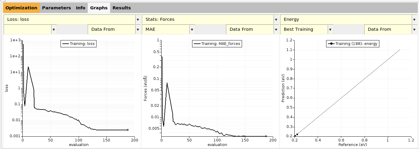
Go to the Graphs panel. There are three curves shown:
The loss function vs. evaluation number
The RMSE (root mean squared error) of energy predictions vs. evaluation number
A scatter plot of predicted vs. reference energies
There are many different types of graphs that you can plot. To plot a correlation plot between the predicted and reference forces:
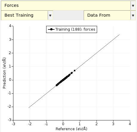
The black diagonal line is the line y = x. In this case, the predicted forces are very close to the reference forces! Let’s compare to the initially predicted forces, i.e. let’s compare the optimized parameters eps = 0.000196 and rmin = 3.6538 (from evaluation 144) to the initial parameters eps = 0.0003 and rmin = 4.0 (from evaluation 0):
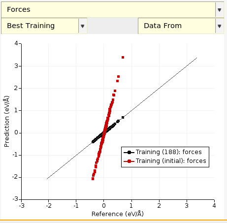
There is a third drop-down where you can choose whether to plot the Best or Latest training data. In this example, both correspond to evaluation 144. In general, the latest evaluation doesn’t have to be the best. This is especially true for other optimizers like the CMA optimizer (recommended for ReaxFF).
Go to the directory results/optimization/training_set_results/best/scatter_plots, and run
"$AMSBIN"/params plot forces.txt
This creates a plot similar to the one shown in the beginning of this tutorial.
For details, see the ParAMS Python examples.
2.2.6.3. Error plots
Go to the Graphs panel.
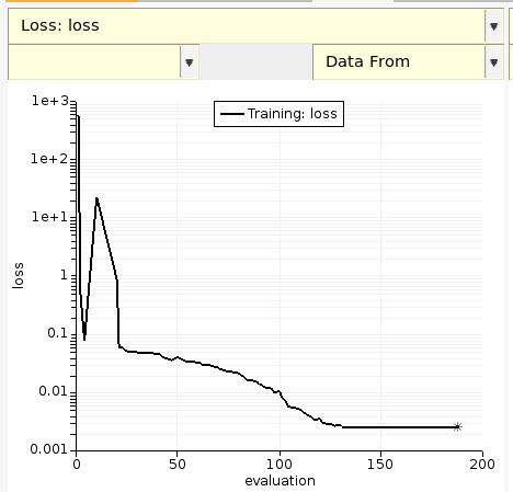
The left-most plot shows the evolution of the loss function with evaluation number. The goal of the parametrization is to minimize the loss function.
By default, the loss function value is saved every 10 evaluations or whenever it decreases.
You can also choose between the RMSE and MAE (mean absolute error) for energies and forces (and other predicted properties):
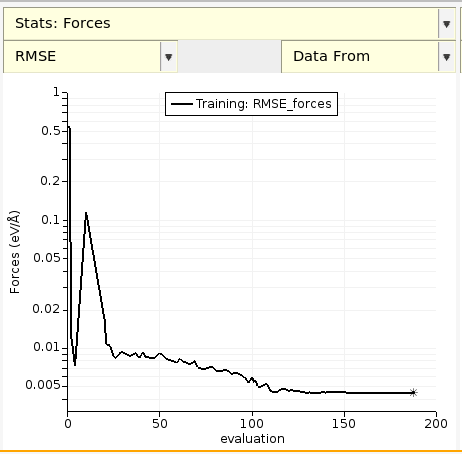
By default, the RMSE and MAE are saved every 10 evaluations or whenever the loss function decreases.
In the results/optimization/training_set_results/ directory are two files running_loss.txt and running_stats.txt.
These files can easily be imported into a spreadsheet (Excel) for plotting, or plotted with, for example, gnuplot.
For details, see the ParAMS Python examples.
2.2.6.4. Parameter plots
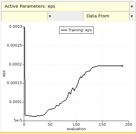
The parameters are by default saved every 500 evaluations, or whenever the loss function decreases.
You can similarly plot the rmin parameter.
Mouse-over the graph to see the value of the parameter at that iteration.
The best parameter values are shown on the Parameters tab.
The file results/optimization/training_set_results/running_active_parameters.txt contains the parameter values vs. evaluation number.
As before, this can be plotted using ParAMS:
"$AMSBIN"/params plot running_active_parameters.txt
For details, see the ParAMS Python examples.
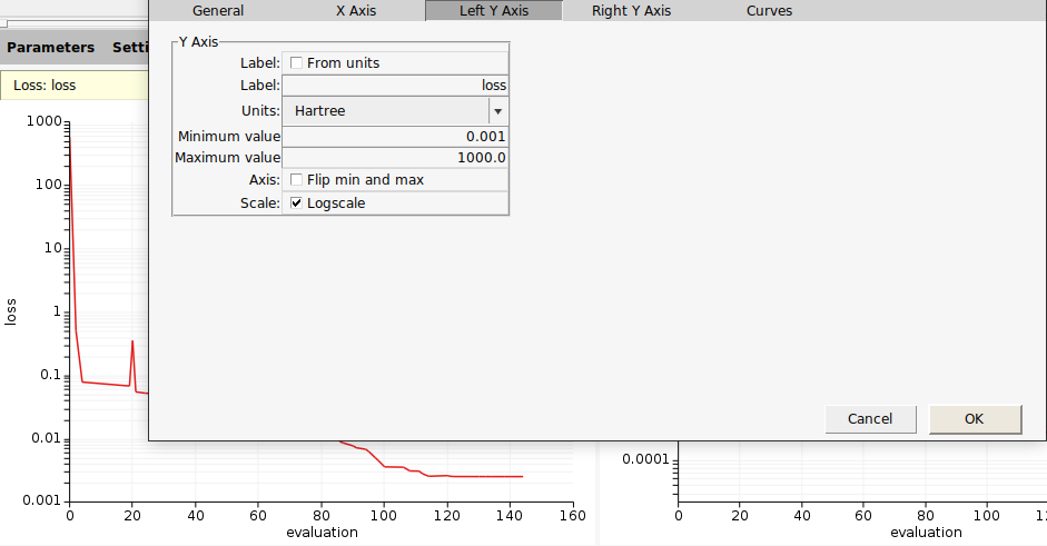
2.2.6.5. Editing and Saving Plots
All of the above GUI plots can be customized to your liking by double clicking anywhere on one of the plot axes. This brings up a window allowing you to configure various graph options like scales, labels, limits, titles, etc.
To save the plot:
If you would like to extract the raw data from the plot in .xy format:
2.2.6.6. Predicted values
Switch to the Training Set panel in the upper table.
The Prediction column contains the predicted values (for the best evaluation, i.e., the one with the lowest loss function value). For the forces, only a summary of the minimum and maximum value is given. To see all predicted, values select one of the Forces entries and go to the Info panel at the bottom and scroll down.
You can also view the predicted values in a different way:
lennardjones.results/optimization/training_set_results/best/scatter_plots/energy.txt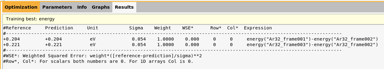
This shows a good agreement between the predicted and reference values for the relative energies in the training set.
lennardjones.results/optimization/training_set_results/best/scatter_plots/forces.txt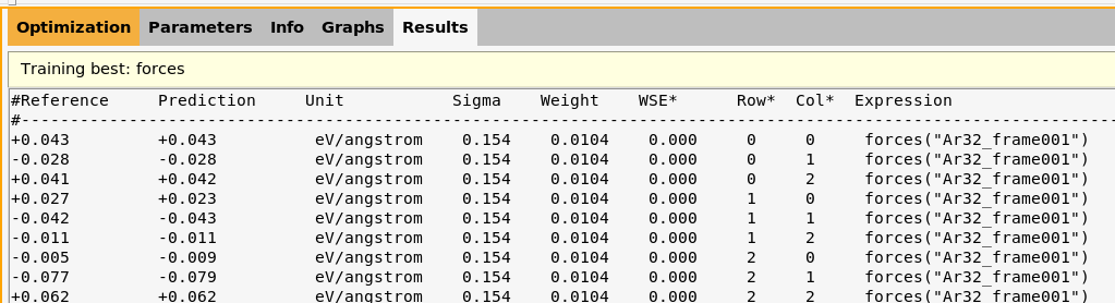
energy.txt and forces.txt are the files that are plotted when making Correlation plots.
There is one file for every extractor in the training set.
The predicted values can be viewed in:
results/optimization/training_set_results/best/data_set_predictions.yaml. This file has the same format as training_set.yaml, but contains also the predicted values.results/optimization/training_set_results/best/scatter_plots/energy.txt(orforces.txt).
For example, the latter file contains
#Reference     Prediction     Unit           Sigma    Weight    WSE*      Row*  Col*  Expression
#------------------------------------------------------------------------------------------------------------------------
+0.204         +0.204         eV             0.054    1.0000    0.000     0     0     energy('Ar32_frame001')-energy('Ar32_frame002')
+0.221         +0.221         eV             0.054    1.0000    0.000     0     0     energy('Ar32_frame003')-energy('Ar32_frame002')
#------------------------------------------------------------------------------------------------------------------------
#WSE*: Weighted Squared Error: weight*([reference-prediction]/sigma)**2
#Row*, Col*: For scalars both numbers are 0. For 1D arrays Col is 0.
This shows a good agreement between the predicted and reference values for the relative energies in the training set.
For details, see the ParAMS Python examples and the documentation for Data Set Evaluator.
2.2.6.7. Loss contributions
In the top table, switch to the Training Set panel.
The last column Loss % contains the Loss Contribution. For each training set entry, it gives the fraction that the entry contributes to the loss function value.
Here, for example, the two Energy entries only contribute 0.96% to the loss function, and the three Forces entries contribute 99.04%. If you notice that some entries have a large contribution to the loss function, and that this prevents the optimization from progressing, you may consider decreasing the weight of those entries.
The loss contribution is printed in the files
results/optimization/training_set_results/best/data_set_predictions.yamlresults/optimization/training_set_results/best/stats.txt
For details, see the ParAMS Python examples and the documentation for Data Set Evaluator.
2.2.6.8. Summary statistics
lennardjones.results/optimization/training_set_results/best/stats.txt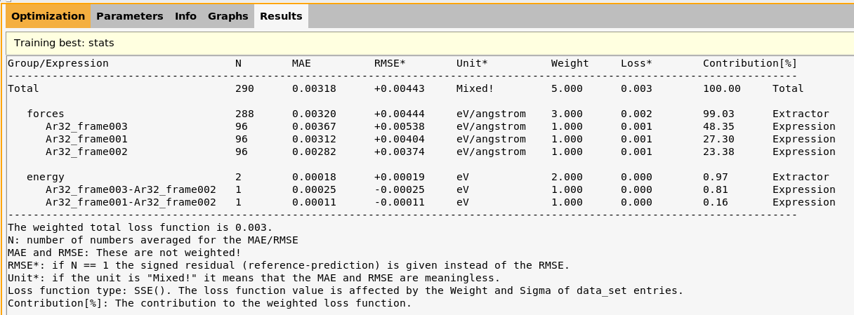
Open the file results/optimization/training_set_results/best/stats.txt
Group/Expression                    N        MAE          RMSE*        Unit*          Weight     Loss*        Contribution[%]
-----------------------------------------------------------------------------------------------------------------------------
Total                               290      0.00318      +0.00443     Mixed!         5.000      0.003        100.00     Total

   forces                           288      0.00320      +0.00444     eV/angstrom    3.000      0.002        99.03      Extractor
      Ar32_frame003                 96       0.00367      +0.00538     eV/angstrom    1.000      0.001        48.34      Expression
      Ar32_frame001                 96       0.00312      +0.00404     eV/angstrom    1.000      0.001        27.31      Expression
      Ar32_frame002                 96       0.00282      +0.00374     eV/angstrom    1.000      0.001        23.38      Expression

   energy                           2        0.00018      +0.00019     eV             2.000      0.000        0.97       Extractor
      Ar32_frame003-Ar32_frame002   1        0.00024      -0.00024     eV             1.000      0.000        0.80       Expression
      Ar32_frame001-Ar32_frame002   1        0.00011      -0.00011     eV             1.000      0.000        0.16       Expression
-----------------------------------------------------------------------------------------------------------------------------
The weighted total loss function is 0.003.
N: number of numbers averaged for the MAE/RMSE
MAE and RMSE: These are not weighted!
RMSE*: if N == 1 the signed residual (reference-prediction) is given instead of the RMSE.
Unit*: if the unit is "Mixed!" it means that the MAE and RMSE are meaningless.
Loss function type: SSE(). The loss function value is affected by the Weight and Sigma of data_set entries.
Contribution[%]: The contribution to the weighted loss function.
For details, see the ParAMS Python examples and the documentation for Data Set Evaluator.
This file gives the mean absolute error (MAE) and root-mean-squared error (RMSE) per entry in the training set. The column N gives how many numbers were averaged to calculate the MAE or RMSE.
For example, in the row forces the N is 288 (the total number of force components in the training set), and the MAE taken over all force components is 0.00320 eV/Å. In the row Ar32_frame003, the N is 96 (the number of force components for job Ar32_frame003), and the MAE is 0.00367 eV/Å.
Further down in the file are the energies. In the row energy the N is 2 (the total number of energy entries in the training set). The entry Ar32_frame003-Ar32_frame002 has N = 1, since the energy is just a single number. In that case, the MAE and RMSE would be identical, so the file gives the absolute error in the MAE column and the signed error (reference - prediction) in the RMSE column.
The file also gives the weights, loss function values, and loss contributions of the training set entries. The total loss function value is printed below the table.
2.2.6.9. All output files
The GUI stores all results in the directory jobname.results (here lennardjones.results).
The results from the optimization are stored in the optimization directory. All the inputs to the optimization are stored in the settings_and_initial_data directory:
jobname.results
├── settings_and_initial_data
│   └── data_sets
└── optimization
    ├── summary.txt
    ├── glompo_optimizer_printstreams
    ├── optimizer_001
    │   ├── end_condition.txt
    │   └── training_set_results
    │       ├── best
    │       │   ├── pes_predictions
    │       │   └── scatter_plots
    │       ├── history
    │       │   ├── 000000
    │       │   │   ├── pes_predictions
    │       │   │   └── scatter_plots
    │       │   └── 000144
    │       │       ├── pes_predictions
    │       │       └── scatter_plots
    │       └── latest
    │           ├── pes_predictions
    │           └── scatter_plots
    └── training_set_results
        ├── best
        │   ├── pes_predictions
        │   └── scatter_plots
        ├── initial
        │   ├── pes_predictions
        │   └── scatter_plots
        └── latest
            ├── pes_predictions
            └── scatter_plots
The
settings_and_initial_datadirectory contains compressed versions of the job collection, training set, and parameter interface. It also contains a detailedparams.infile representing the chosen optimization settings. This directory is a totally self-contained copy of all the optimization inputs and can be shared, archived or used to rerun the job on other machines.From AMS2023, ParAMS can start multiple optimizers during a single optimization. The results from each optimizer will be placed in a directory labelled
optimizer_xxx, wherexxxis the unique optimizer identification number. Such folders contain anend_condition.txtfile detailing the reason they stopped, and directories for each of the data sets being evaluated. In this case, only thetraining_setwas used.The
optimization/training_set_resultsdirectory contains global detailed results for thetraining set, combined across all optimizers.
The training_set_results directories contain the following:
The running_loss.txt file records the loss function value, evaluation number, time, and (in the global results) the optimizer which did the evaluation.
The running_active_parameters.txt file records the parameter values per evaluation number.
The running_stats.txt file records the MAE and RMSE per extractor vs. evaluation number.
The
bestsubdirectory contains detailed results for the iteration with the lowest loss function value (globally or for a specific optimizer).The
historysubdirectory contains detailed results that are stored regularly during the optimization (by default every 500 iterations). Only optimizer specific results havehistorydirectories.The
initialsubdirectory contains detailed results for the first iteration (with the initial parameters). Only the global level results have theinitialdirectory.The
latestsubdirectory contains detailed results for the latest iteration.
In this tutorial, only one optimizer was started, so the contents of the global level results and optimizer_001 will be the same.
Further, both the best and latest evaluations were evaluation 144, your results will likely have a different number.
In general, the latest evaluation doesn’t have to be the best.
This is especially true for other optimizers like the CMA optimizer (recommended for ReaxFF).
Each detailed result subdirectory contains the following:
active_parameters.txt: List of the active parameter valuesdata_set_predictions.yaml : File storing the training set with both the reference values and predicted values.
engine.txt: an AMS Engine settings input block for the parameterized engine.evaluation.txt: the evaluation numberoptimizer_id.txt: the number of the optimizer which produced the result (global level only)lj_parameters.txt: The parameters in a format that can be read by AMS. Here, it is identical to engine.txt. For ReaxFF parameters, you instead get a fileffield.ff. For GFN1-xTB parameters, you get a folder calledxtb_files.loss.txt: The loss function valueparameter_interface.yaml: The parameters in a format that can be read by ParAMSpes_predictions: A directory containing results for PES scans: bond scans, angle scans, and volume scans. It is empty in this tutorial. For an example, see ReaxFF (basic): H₂O bond scan.scatter_plots: Directory containing
energy.txt,forces.txt, etc. Each file contains a table of reference and predicted values for creating scatter/correlation plots.stats.txt: Contains MAE/RMSE/Loss contribution for each training set entry sorted in order of decreasing loss contribution.
2.2.6.10. summary.txt
The results/optimization/summary.txt file contains a summary of the job collection, training set, and settings:
Optimization() Instance Settings:
=================================
Workdir:                           LJ_Ar/optimization/optimization
JobCollection size:                3
Interface:                         LennardJonesParameters
Active parameters:                 2
Optimizer:                         Scipy
Parallelism:                       ParallelLevels(optimizations=1, parametervectors=1, jobs=1, processes=1, threads=1)
Verbose:                           True
Callbacks:                         Logger
                                   Timeout
                                   Stopfile
PLAMS workdir path:                /tmp

Evaluators:
-----------
Name:                              training_set (_LossEvaluator)
Loss:                              SSE
Evaluation interval:              1

Data Set entries:                  5
Data Set jobs:                     3
Batch size:                        None

Use PIPE:                          True
---
===
Start time: 2021-12-06 10:07:21.681185
End time:   2021-12-06 10:07:32.125530
2.2.7. Close the ParAMS GUI
When you close the ParAMS GUI (File → Close), you will be asked whether to save your changes.
This question might appear strange since you didn’t make any changes after running the job.
The reason is that ParAMS auto-updates the table of parameters while the parametrization is running, and also automatically reads the optimized parameters when you open the project again. To revert to the initial parameters, choose File → Revert Parameters.
If you save the changes, this will save the optimized parameters as the “new” starting parameters, which could be used as a starting point for further parametrization.
We do not recommend to overwrite the same folder several times with different starting parameters. Instead, if you want to save after having made changes to the parameters, use File → Save As and save in a new directory.
2.2.8. Appendix: Creation of the input files
How to run the reference calculations and import the results into ParAMS is explained in the Import training data (GUI) tutorial. The data for this Lennard-Jones tutorial was generated following the section MD with fast method followed by Replay with reference method.
The AMS Input language is human-readable, thus, the params.in can be written manually.
The parameter_interface.yaml, job_collection.yaml, training_set.yaml files were created with a
script combining functionality from PLAMS and
ParAMS. Download the script if you would like to try it. It sets
up a molecular dynamics simulation of liquid Ar with the UFF force field. Some
snapshots are recalculated with dispersion-corrected DFTB (GFN1-xTB). A
ResultsImporter then extracts the forces and relative energies, and
creates the job_collection.yaml and training_set.yaml files.
2.2.9. Next steps
Learn about running multiple optimizers at once.
Try the ReaxFF (basic): H₂O bond scan or GFN1-xTB: Lithium fluoride tutorial.
Learn how to import your own training data into ParAMS. If you already have a ReaxFF training set for use with AMS up to version 2021, it can be directly converted to ParAMS format
Learn more about training and validation sets.