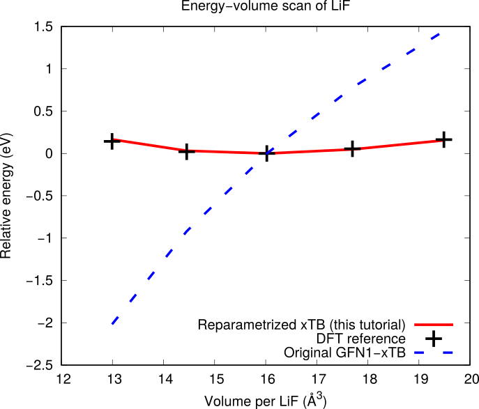
3.5. GFN1-xTB: Lithium fluoride
This example refits the Li and F repulsive potentials of the GFN1-xTB model, available in AMS under the DFTB engine. With GFN1-xTB, a lattice optimization of LiF in the rock salt structure collapses the unit cell, because the Li-F interaction is not repulsive enough. This motivates the reparametrization.
Expt. |
GFN1-xTB |
Reparametrized xTB (this tutorial) |
|
LiF enthalpy of formation (eV) |
-6.394 |
-8.143 |
-6.393 |
The fitting is done to better reproduce:
DFT-calculated energy-volume curve of LiF
Optionally, the stress tensors for each point along the energy-volume curve
experimental enthalpy of formation for LiF [reaction enthalpy for ½ F₂(g) + Li(s) → LiF(s)]
experimental bond length of F₂ (1.41 Å).
The tutorial will also teach you how you can use different k-space samplings (GFN1-xTB settings) for different jobs.
Note
The input files have already been prepared. If you simply want to run the
parametrization without preparing the input, copy the contents of
$AMSHOME/scripting/scm/params/examples/xTB_LiF to a new empty
directory.
To open the example in the graphical user interface (GUI): SCM → ParAMS,
File → Open the job_collection.yaml file in the new directory.
You can then run the parametrization.
3.5.1. Energy-volume scan reference calculation for LiF
Note
The calculation below uses the BAND periodic DFT engine. If you do not have
a license for BAND, or want a faster reference calculation for this
tutorial, you could instead run the reference calculation using a different
DFTB model ( panel, Model → SCC-DFTB, Parameters →
QUASINANO2015). You would then fit one DFTB model (xTB) to reference data
calculated with another (SCC-DFTB).
panel, Model → SCC-DFTB, Parameters →
QUASINANO2015). You would then fit one DFTB model (xTB) to reference data
calculated with another (SCC-DFTB).
First, import the structure and set the DFT settings in AMSinput:
LiF_primcell.xyz into AMSinput panel
panel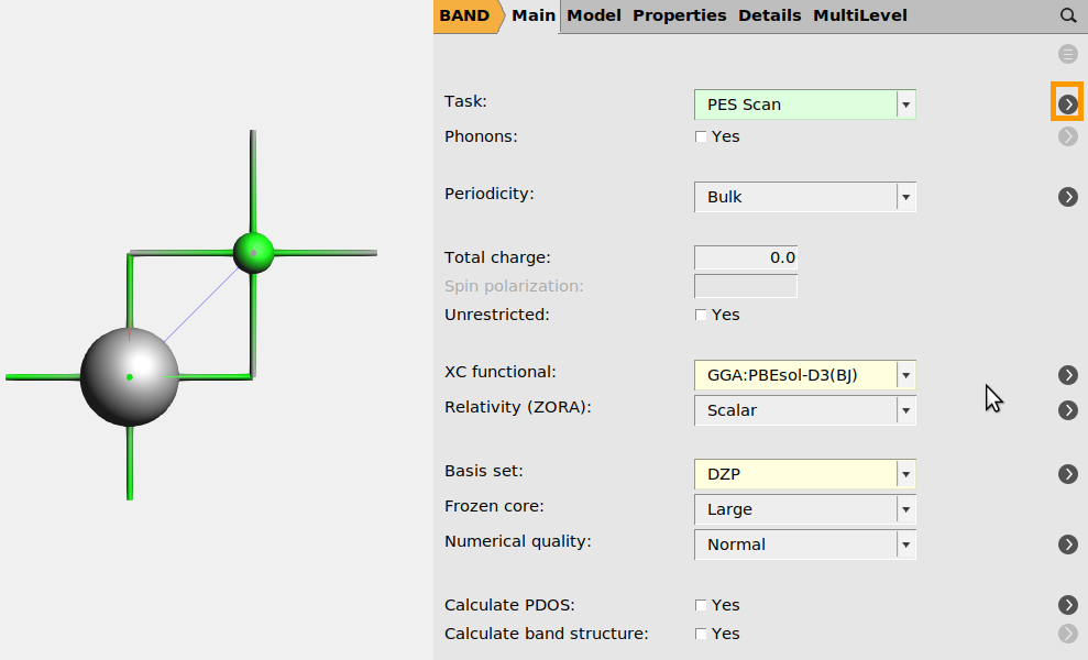
Note
For energy-volume scans it is often a good idea to use more dense k-space sampling. Here, we keep the numerical quality at Normal only to have the calculation finish faster. (If you want an even faster calculation, set Numerical Quality to Basic).
Then, set up the energy-volume scan:
 button next to Cell volume
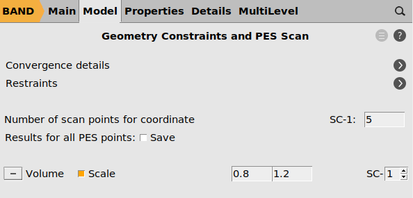
Optionally (this will make the calculation more expensive but provide more training data), calculate the stress tensor for each volume:
Save with the name volumescan.ams and run the calculation. Note that it may
take about an hour to finish, or more if you enabled the stress tensor
calculation (depending on your hardware).
Tip
While the calculation is running you can continue with the step Import experimental formation enthalpy into ParAMS.
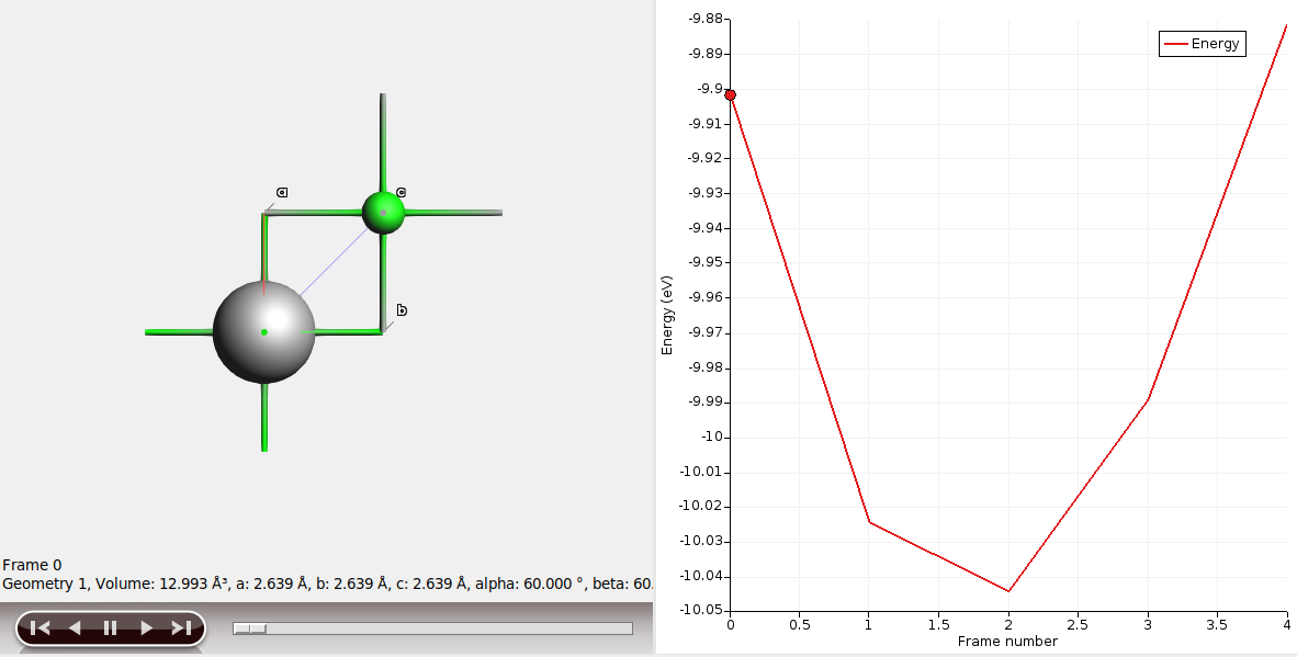
When the calculation has finished, see the energy as a function of volume by either
opening the calculation in AMSmovie, or
selecting the job in AMSjobs, and running Tools → Build Spreadsheet
The function run_reference in generate_input_files.py sets up and runs the job via PLAMS:
def run_reference(xyz_file):
"""
Sets up a volume scan of LiF with PBEsol-D3(BJ).
For each point, the stress tensor is calculated.
Returns the path to the ams.rkf file
NOTE: This is an expensive calculation that might take several hours.
"""
init()
mol = Molecule(xyz_file)
s = Settings()
s.input.band.KSpace.Type = "Symmetric"
s.input.band.KSpace.Quality = "Normal" # N.B. this should be set to 'Good' for production calculations!
s.input.band.XC.GGA = "PBEsol"
s.input.band.XC.Dispersion = "Grimme3 BJDamp"
s.input.band.Basis.Type = "DZP"
s.input.ams.Task = "pesscan"
s.input.ams.PESScan.ScanCoordinate.NPoints = 5
s.input.ams.PESScan.ScanCoordinate.CellVolumeScalingRange = "0.80 1.20"
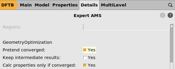
s.input.ams.PESScan.CalcPropertiesAtPESPoints = "Yes" # needed to get the stress tensor at each point
s.input.ams.GeometryOptimization.MaxIterations = 0
s.input.ams.GeometryOptimization.PretendConverged = "Yes"
s.input.ams.Properties.StressTensor = "Yes"
job = AMSJob(settings=s, molecule=mol, name="volumescan")
job.run()
finish()
return job.results.rkfpath()
3.5.2. Import the energy-volume scan into ParAMS
First, open ParAMS in GFN1-xTB mode:
Then, import the results from the reference job:
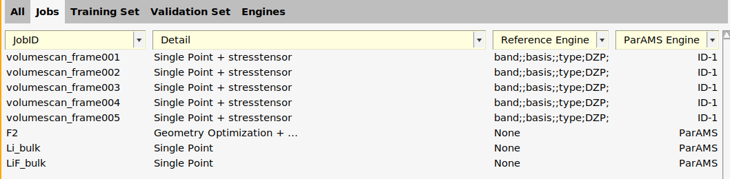
volumescan.results)relative_energiesstresstensor_diagonal_3d. Note: You can choose several entries in the drop-down list!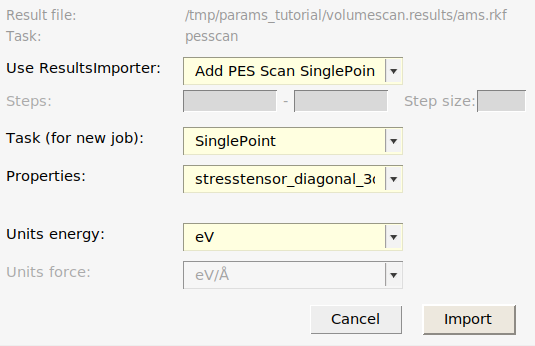
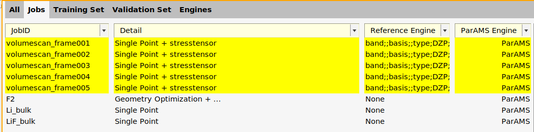
This creates 5 singlepoint jobs to be run during the optimization.
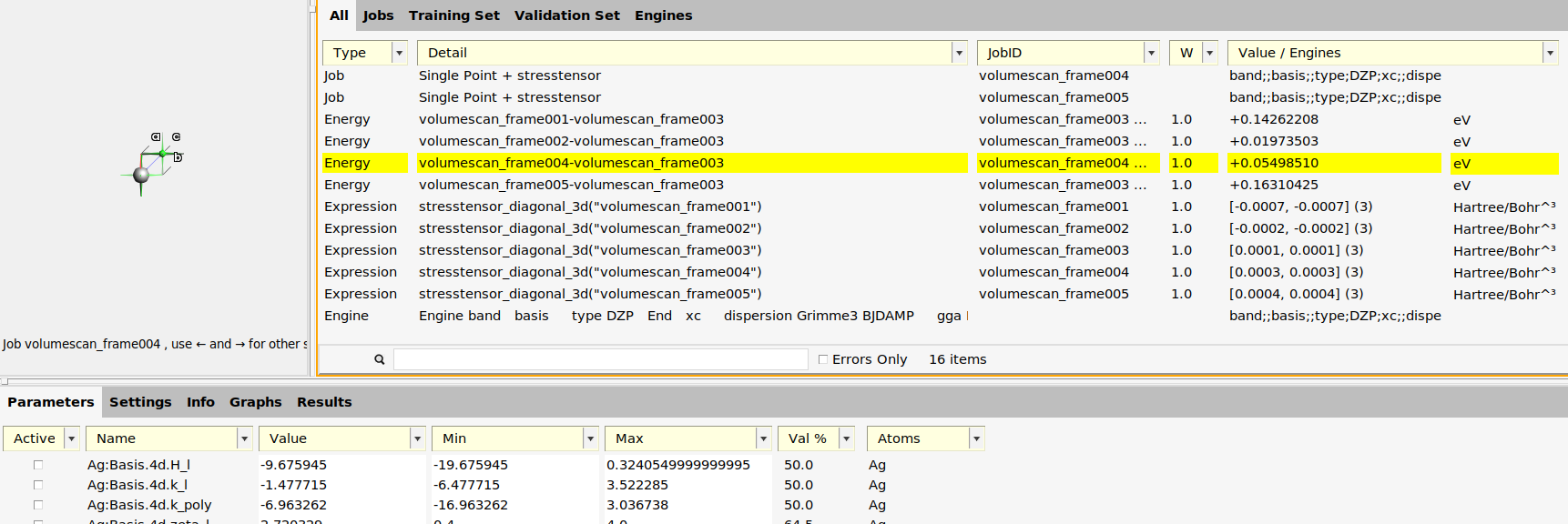
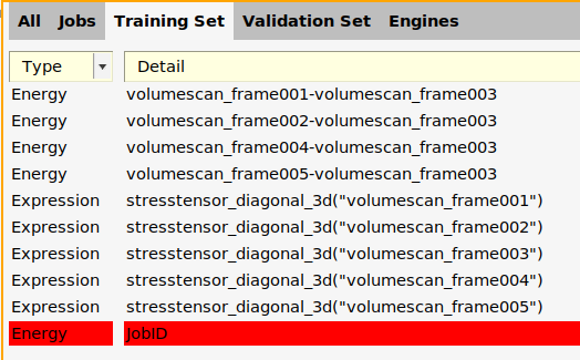
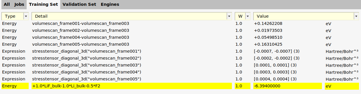
The training set contains 4 relative energies: volumescan_frame001-volumescan_frame003, …, volumescan_frame005-volumescan_frame003. The energies are taken relative to frame 3, which is the lowest energy frame.
It also (optionally) contains 5 stress tensors, one for each frame. The
stresstensor_diagonal_3d property only extracts the diagonal elements of
the stress tensor for a 3D system. To also include the off-diagonal elements,
you could have checked the stresstensor_3d option in the importer dialog.
Note
It is currently not possible to set a custom unit for the stress tensor in the GUI, but it is possible using scripting. The default unit for the stress tensor is hartree/bohr³.
Save your work before continuing:
LiF.paramsThe function add_volume_scan in generate_input_files.py uses a Results Importer as follows:
def add_volume_scan(results_importer: ResultsImporter, ref_rkf: str):
    """
    The volume scan is added using the add_pesscan_singlepoints() method, which supports extracting the stress tensor.

    If no stress tensor is desired, an alternative is to instead use the add_singlejob() method with task='PESScan'

    See the documentation for more details.
    """
    results_importer.add_pesscan_singlepoints(
        ref_rkf,
        properties={
            "relative_energies": {
                "relative_to": "min",
                "unit": "eV",
            },
            "stresstensor_diagonal_3d": {
                "unit": "GPa",
            },
        },
        extra_engine="kspace_normal_symmetric",
    )
Here, the extra_engine='kspace_normal_symmetric' option is used to specify job-dependent engine settings.
Note
There are two different params results importers that work on PES scans: add_singlejob and add_pesscan_singlepoints.
The stress tensor can only be imported using add_pesscan_singlepoints and is the results importer used above.
If you did not calculate the stress tensor at each point, you can use the add_singlejob results importer with the pes extractor. That will produce the types of energy-volume curves shown in the ReaxFF (advanced): ZnS tutorial. For more information, see PES scans: bond scan, angle scan, or volume scan.
3.5.3. Import experimental formation enthalpy into ParAMS
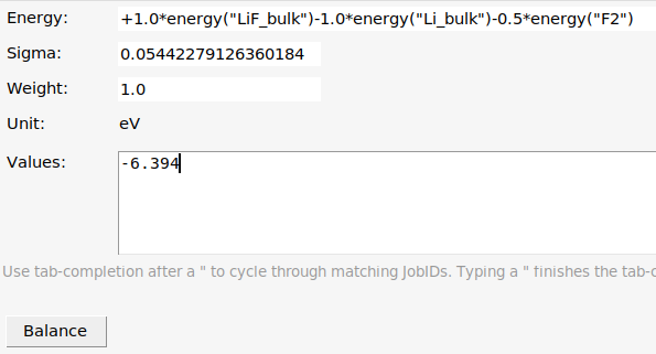
ParAMS can be used to train to experimental reference data. In that way, you do not need to run expensive DFT reference calculations. Here, we demonstrate it for LiF. The reaction
½ F₂ (g) + Li(s) → LiF(s)
has ΔH⁰ = -617 kJ/mol = -147 kcal/mol = -0.2350 Ha = -6.394 eV. Let’s add this reaction energy to the training set.
First, let’s add a geometry optimization job for F₂(g), and two single point jobs for Li(s) and LiF(s). Li has the body-centered cubic (bcc) structure, and LiF has the NaCl (rock salt) structure.
panel. next to Geometry Optimization
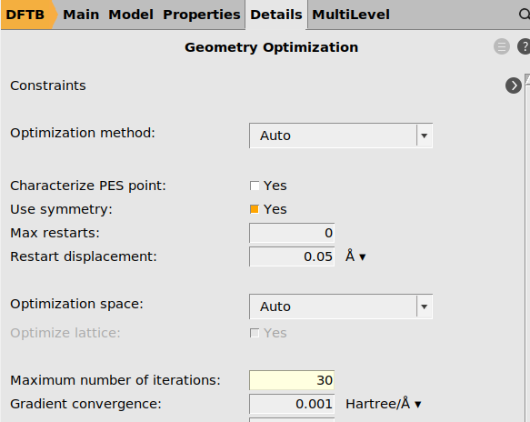
f and click the positions of the two atoms. Or use the  periodic table to select fluorine.
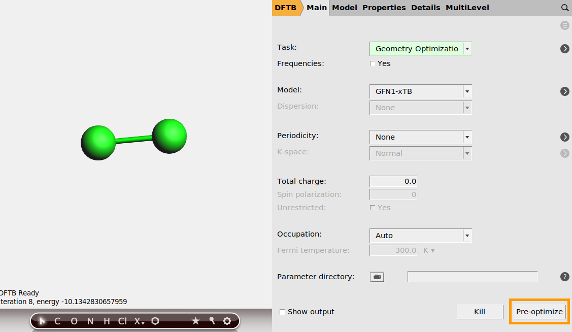
F2.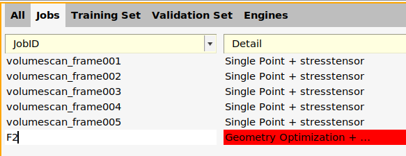
The added job F2 is a Geometry Optimization job, meaning that the geometry will be optimized for every set of parameter values during the parametrization.
We now perform similar steps for Li and LiF, but add them as SinglePoint jobs:
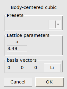
Li_bulk.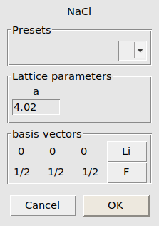
LiF_bulk.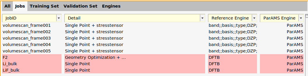
Note that the Reference Engine column says DFTB - it corresponds to the settings used in AMSinput. It can be used to use ParAMS to calculate reference values. However, in this tutorial we will use experimental reference data. Therefore, let’s delete the reference engine from the three new entries.
F2 job (where it says Geometry Optimization + ...).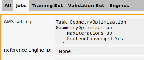
Li_bulk and LiF_bulk jobs.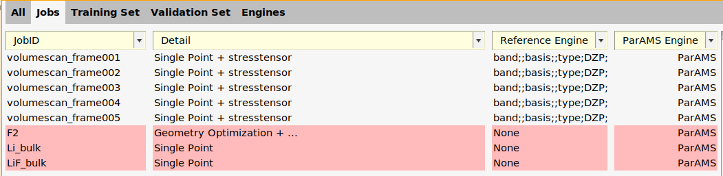
Now you can add a reaction energy:
1.0*energy("LiF_bulk")-energy("Li_bulk")-energy("F2")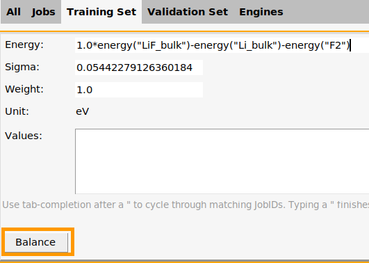
Tip
When typing energy expressions, you can use tab-completion. For example, if you start typing energy("Li and press TAB multiple times, you will cycle through energy("Li_bulk") and energy("LiF_bulk").
The function add_enthalpy_of_formation in generate_input_files.py uses the Results Importer add_reaction_energy. The needed .xyz files can be found in $AMSHOME/scripting/scm/params/examples/xTB_LiF.
def add_enthalpy_of_formation(results_importer: ResultsImporter):
    """
    Adds experimental enthalpy of formation of LiF
    The jobs are added with Good k-space quality, since total energies of different
    supercells are sensitive to the k-space sampling. (Moreover Li is a metal)
    """
    LiF = Molecule("LiF_primcell.xyz")
    Li = Molecule("Li_primcell.xyz")
    F2 = Molecule("F2.xyz")
    results_importer.add_reaction_energy(
        reactants=[Li, F2],
        reactants_names=["Li_bulk", "F2"],
        products=[LiF],
        products_names=["LiF_bulk"],
        normalization="p0",  # reaction energy per LiF (first product)
        task="GeometryOptimization",
        reference=-6.394,
        unit="eV",
        extra_engine="kspace_good_symmetric",  # applied to the Li_bulk and LiF_bulk jobs. The F2 molecule is nonperiodic so the k-space settings are ignored
    )
The extra_engine option specifies the DFTB settings to be used during the parametrization.
Important
When adding the reference value manually, verify that the stoichiometric
coefficients are correct. Here, the Li_bulk job contains one formula
unit of Li (the primitive Li unit cell), the LiF_bulk job has one
formula unit of LiF (the primitive LiF unit cell), and F2 has one
formula unit of F₂. This means that the chemical systems perfectly match
the species in the chemical equation.
However, if you for example were to import the conventional unit cell of LiF, which has 4 LiF formula units (Li₄F₄), then the reaction would be written as
½ F₂(g) + Li(s) → ¼ Li₄F₄(s), ΔH⁰ = -617 kJ/mol
or
2 F₂(g) + 4 Li(s) → Li₄F₄(s), ΔH⁰ = -2468 kJ/mol
Note
The above box shows two different ways of writing the same reaction, with different reaction energies. During the parametrization, the error of the predicted reaction energy will be 4 times larger if you use the second equation (ΔH⁰ = -2468 kJ/mol). That will implicitly make this training set entry more important, at the expense of other training set entries.
Set Sigma to what you think would be an acceptable error for your reaction energies, and set Weight to how important you consider the training set entry to be.
See also: Sigma vs. weight: What is the difference?.
3.5.4. Import experimental F₂ bond length
For the F2 geometry optimization job from the previous section, we can add another training set entry.
F2 job.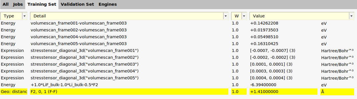
The add_bond_length function in generate_input_files.py:
def add_bond_length(results_importer: ResultsImporter):
    """add experimental F2 bond length. This requires that the job F2 has been defined (which is done in add_enthalpy_formation)"""
    results_importer.data_set.add_entry('distance("F2",0,1)', reference=1.41)
This function adds an entry to the dataset with the distance extractor. See also: Demonstration: Working with a DataSet
3.5.5. Job-dependent engine settings (k-space)
GFN1-xTB is an electronic structure method. For periodic crystals, it is important to converge the k-space sampling, especially if the energies of the jobs are used. In this tutorial, both the energy-volume scan and the formation enthalpy make use of the energies, and compare energies for different lattices. What should the k-space samplings be for those jobs?
It is up to you to decide. Here, we will demonstrate how to set a Good
k-space quality for the Li_bulk and LiF_bulk jobs, and how to use Normal
k-space quality for the volume scan jobs. For F2 (gas-phase), the k-space
settings are ignored.
We set KSpace Type to Symmetric, because the systems (primitive unit cells of Li and LiF) are very symmetric (it is faster than a Regular grid).
See also
k-space documentation for more details about k-point grids (Regular, Symmetric, Quality, NumberOfPoints, …)
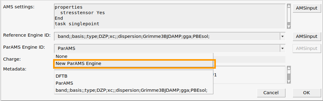
In the GUI, the engine settings during the parametrization are referred to as “ParAMS Engines” (in contrast to settings used for reference calculations, that are referred to as reference engines).
There is always a ParAMS engine called ParAMS, which uses the default engine settings.
We will create two new ParAMS engines
kspace_normal_symmetric : KSpace Type Symmetric and KSpace Quality Normal
kspace_good_symmetric : KSpace Type Symmetric and KSpace Quality Good
 main panel, set Periodicity to Bulk. This activates the k-space options. arrow next to K-space.
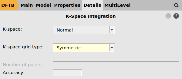
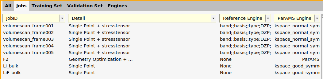
In the Jobs panel, the ParAMS engine is now given as ID-1 for the volumescan jobs.
We can give the engine a more descriptive name:
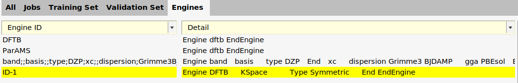
ID-1 to kspace_normal_symmetric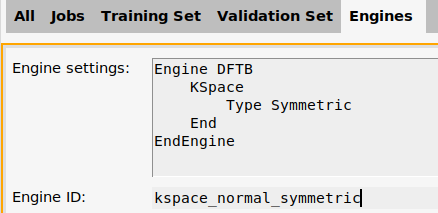
On the Jobs panel, the ParAMS Engine ID has also been updated:
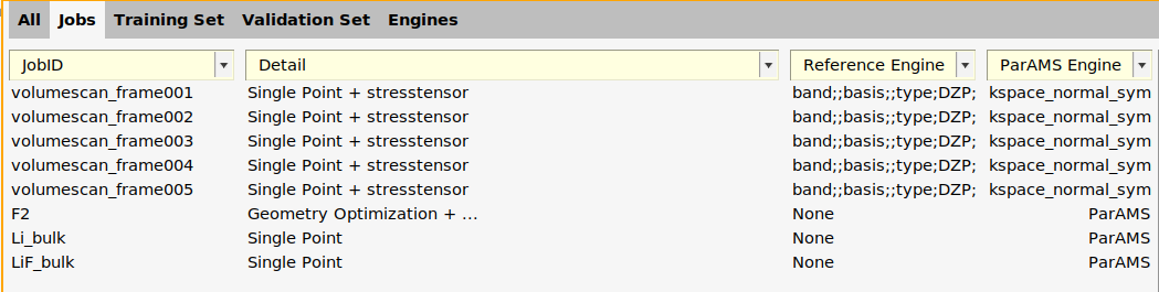
Warning
When you select many jobs, double-click in the details column, and make any changes, all settings (AMS settings, Reference Engine ID, and ParAMS Engine ID) will be copied to the selected jobs.
Tip
If you have many jobs, use the search box at the bottom of the table to
filter. For example, type volumescan to only see the jobs matching
volumescan. Remember to clear the search box to see all jobs again.
LiF_bulk and Li_bulk jobs. Select the jobs, double-click in the Details column, create a new ParAMS engine, set K-space grid type to Symmetric and the Quality to Good. Name the engine kspace_good_symmetric.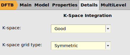
The function add_engines in generate_input_files.py adds two new engines to the Engine Collection:
def add_engines(results_importer: ResultsImporter):
    """Control the k-space settings for each job by adding different engine definitions."""
    s = Settings()
    s.input.dftb.KSpace.Type = "Symmetric"
    s.input.dftb.KSpace.Quality = "Normal"
    results_importer.job_collection.engines.add_entry("kspace_normal_symmetric", Engine(s))

    s = Settings()
    s.input.dftb.KSpace.Type = "Symmetric"
    s.input.dftb.KSpace.Quality = "Good"
    results_importer.job_collection.engines.add_entry("kspace_good_symmetric", Engine(s))
The labels 'kspace_normal_symmetric' and
'kspace_good_symmetric' can be referred to using the
extra_engine argument when calling a results importer. See the
previous examples above.
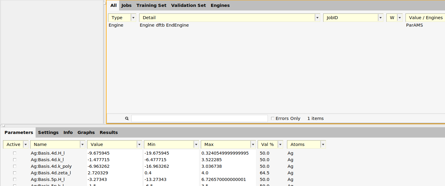
3.5.6. Set parameters to optimize and their ranges
In xTB, the repulsive potential is controlled by the two parameters alpha and Z for each element.
F: in the search box.F:Z and F:alpha.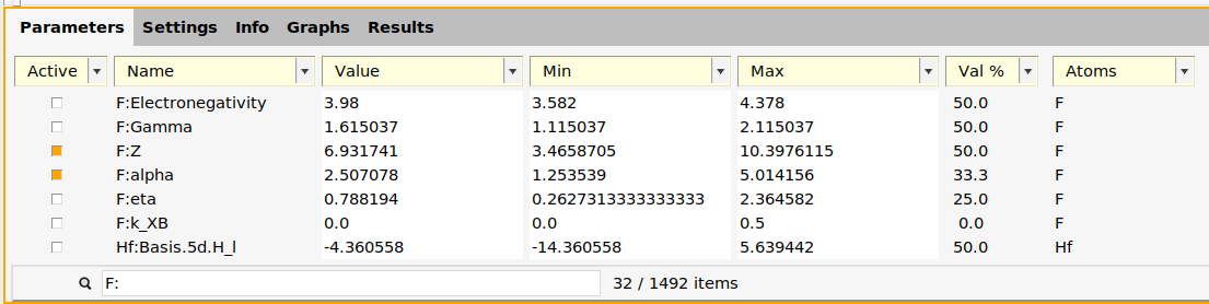
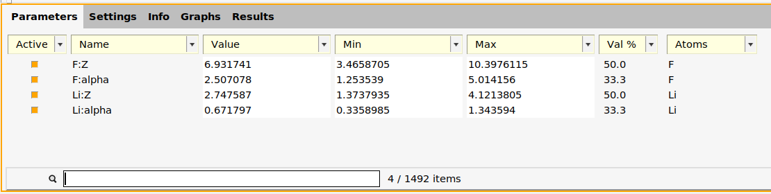
Li: in the search boxLi:Z and Li:alpha.Optionally, you can also change the minimum and maximum allowed values of the parameters by changing the numbers in the Min and Max columns.
Double-check that only the four parameters F:Z, F:alpha, Li:Z, and Li:alpha are active:
The function generate_parameter_interface in generate_input_files.py creates the parameter interface.
def generate_parameter_interface():
    """
    Generate parameter_interface.yaml activating
    the Li and F repulsive potentials for optimization
    """
    # s is the *default* engine settings used during the parametrization
    # It is normal to leave it as an empty Settings and set the engine settings per job
    s = Settings()
    interface = GFN1xTBParameters(settings=s)

    # Repulsive potential of Li.
    interface["Li:alpha"].is_active = True
    interface["Li:Z"].is_active = True

    # Repulsive potential of F.
    interface["F:alpha"].is_active = True
    interface["F:Z"].is_active = True

    interface.yaml_store("parameter_interface.yaml")
3.5.7. Set the optimizer settings
 panel
panelThe params.in file contains:
Task Optimization

DataSet
	Name training_set
	Path training_set.yaml
End

LoggingInterval
   General 5
End

ExitCondition
	Type MaxTotalFunctionCalls
	MaxTotalFunctionCalls 400
End

Optimizer
	Type CMAES
	CMAES
		Popsize 8
	End
End
3.5.8. Run the xTB parametrization
Alternatively, select the job in AMSjobs and first choose which queue to run on, before submitting the job.
Use the following command in the directory containing
job_collection.yaml, job_collection_engines.yaml,
parameter_interface.yaml, training_set.yaml, and
params.in:
"$AMSBIN/params"
Depending on your hardware, after about 30-60 minutes you should have obtained a good set of parameters.
Tip
The results will automatically update in the GUI while the parametrization is running.
If you think the results are “good enough”, you do not need to wait for the parametrization to finish. In the GUI, select the job in AMSjobs and choose Job → Request Early Stop to stop the job.
3.5.9. Results of the xTB parametrization
For example,
The optimized parameters are shown on the Parameters tab.
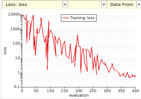
On the Graphs tab you can see the running loss function:
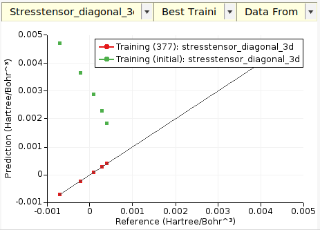
On the Graphs tab you can create a scatter plot of predicted vs. reference stress tensor components, here compared to the original GFN1-xTB:
Tip
You double-click on a plot axis to access plot configuration settings.
On the Results tab you can select Training best: energy to see the energies
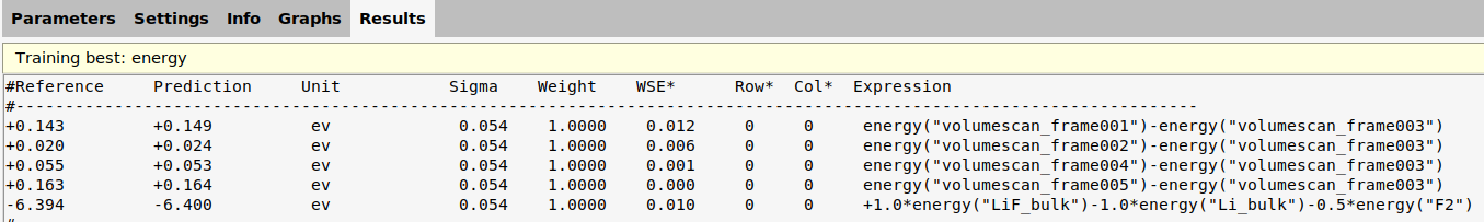
The
xtb_filesdirectory contains all the files needed to run new AMS calculations with the optimized parameters. On the panel in AMSinput, set Model to GFN1-xTB and Parameters directory to the xtb_filesdirectory. If scripting, setEngine DFTB%ResourcesDirto thextb_filesdirectory.xtb_files/elements.xtbparcontains the optimized values of the alpha and Z parameters:
#Element eta Gamma alpha Z k_XB Electronegativity
H 0.470099 0.0 2.2097 1.116244 0.0 2.2
He 1.441379 1.5 1.382907 0.440231 0.0 3.0
Li 0.205342 1.02737 0.3471898244638939 2.481445788775993 0.0 0.98
Be 0.274022 0.900554 0.865377 4.07683 0.0 1.57
B 0.34053 1.3 1.093544 4.458376 0.0 2.04
C 0.479988 1.053856 1.281954 4.428763 0.0 2.55
N 0.476106 0.042507 1.727773 5.498808 0.0 3.04
O 0.583349 -0.005102 2.004253 5.171786 0.0 3.44
F 0.788194 1.615037 2.465746060529967 4.812536210787959 0.0 3.98
See also
Getting Started: Lennard-Jones for more detailed descriptions about the output files and plots.
Note
When using the Add PESScan SinglePoints option, the GUI does not plot
any energy-volume curves (and the pes_predictions folder in the output
is empty). To get such plots, instead use Add SingleJob with the
pes property (see ReaxFF (basic): H₂O bond scan)
You can find some example output files in $AMSHOME/scripting/scm/examples/xTB_LiF/example_output/training_set_results/best.