3.6. DFTB repulsive potential
Note
First go through the Getting Started: Lennard-Jones tutorial.
Note
The ParAMS graphical user interface and the ParAMSJob Python class do not support SCC-DFTB repulsive potentials, but they do support xTB parametrizations. This tutorial uses some internal ParAMS python classes/options that you normally wouldn’t need to use.
This example illustrates how to fit an SCC-DFTB repulsive potential. It is based on the work published in Komissarov et al., J. Chem. Inf. Model. DOI: 10.1021/acs.jcim.1c00333.
Jobs: Lattice optimizations of the wurtzite and rocksalt polymorphs of ZnO
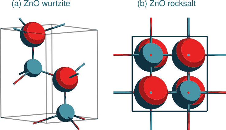
Fig. 3.3 Adapted from Komissarov et al.
Training set: The relative energy between the two polymorphs, and the bulk modulus and optimized lattice parameters of wurtzite. The reference data were calculated with BAND (DFT), using a TZP basis set.
Parameter interface: DFTBSplineRepulsivePotentialParameters
3.6.1. job_collection.yaml and training_set.yaml
All the files needed for this example can be found in $AMSHOME/scripting/scm/params/examples/DFTB_ZnO.
job_collection.yaml: Note that for wurtzite the elastic tensor is calculated, which will also calculate the bulk modulus.
---
ID: rocksalt_lattopt
ReferenceEngineID: None
AMSInput: |
   Task GeometryOptimization
   geometryoptimization
     OptimizeLattice Yes
   End
   system
     Atoms
                Zn      2.1700000000      2.1700000000      2.1700000000
                 O      0.0000000000      0.0000000000      0.0000000000
     End
     Lattice
            0.0000000000     2.1700000000     2.1700000000
            2.1700000000     0.0000000000     2.1700000000
            2.1700000000     2.1700000000     0.0000000000
     End
   End
---
ID: wurtzite_lattopt
ReferenceEngineID: None
AMSInput: |
   Task GeometryOptimization
   geometryoptimization
     OptimizeLattice Yes
     convergence
       Gradients 8e-05
     End
   End
   properties
     ElasticTensor Yes
   End
   system
     Atoms
                Zn      1.6450000000      0.9497411900      0.0233750800
                Zn      0.0000000000      1.8994823900      2.6783750800
                 O      1.6450000000      0.9497411900      3.2953749200
                 O      0.0000000000      1.8994823900      0.6403749200
     End
     Lattice
            3.2900000000     0.0000000000     0.0000000000
           -1.6450000000     2.8492235800     0.0000000000
            0.0000000000     0.0000000000     5.3100000000
     End
   End
...
# 0.5.0
training_set.yaml: The cell_lengths extractor accepts an additional argument: 0 for the first lattice vector (a), and 2 for the third lattice vector (c).
---
Expression: bulkmodulus("wurtzite_lattopt")
Weight: 0.5
Sigma: 10.0
ReferenceValue: 126.193
Unit: GPa, 29421.0152092444
---
Expression: cell_lengths("wurtzite_lattopt", 0)
Weight: 1
ReferenceValue: 3.3029
---
Expression: cell_lengths("wurtzite_lattopt", 2)
Weight: 1
ReferenceValue: 5.3208
---
Expression: energy("wurtzite_lattopt")/2.0-energy("rocksalt_lattopt")
Weight: 1
ReferenceValue: -0.0088641
...
# 0.5.1
3.6.2. Background: znorg-0-1
AMS includes the DFTB.org/znorg-0-1 SCC-DFTB parameters for ZnO. Although
those parameters give good values for the lattice parameters and bulk modulus,
they give the incorrect relative stability of the wurtzite and rocksalt
polymorphs (the “Prediction” numbers were calculated with znorg-0-1):
#Reference     Prediction     Unit           Sigma    Weight    WSE*      Row*  Col*  Expression
#------------------------------------------------------------------------------------------------------------------------
+126.19        +160.88        GPa            10.000   0.5000    6.016     0     0     bulkmodulus("wurtzite_lattopt")
+3.303         +3.290         angstrom       0.050    1.0000    0.065     0     0     cell_lengths("wurtzite_lattopt", 0)
+5.321         +5.376         angstrom       0.050    1.0000    1.237     0     0     cell_lengths("wurtzite_lattopt", 2)
-0.00886       +0.00501       Ha             0.002    1.0000    48.157    0     0     energy("wurtzite_lattopt")/2.0-energy("rocksalt_lattopt")
#------------------------------------------------------------------------------------------------------------------------
#WSE*: Weighted Squared Error: weight*([reference-prediction]/sigma)**2
#Row*, Col*: For scalars both numbers are 0. For 1D arrays Col is 0.
In experiment and DFT, wurtzite is more stable than rocksalt (-0.009 Ha per ZnO formula unit), but with znorg-0-1, the opposite is true (+0.005 Ha per ZnO formula unit). This motivates the reparametrization. The goal of the parametrization is to have wurtzite more stable than rocksalt with the new parameters.
The above table was generated with the following script using a Data Set Evaluator:
from scm.plams import *
from scm.params import *


def main():
    dftb_s = Settings()
    dftb_s.input.dftb.model = "SCC-DFTB"
    dftb_s.input.dftb.kspace.quality = "Good"
    dftb_s.input.dftb.resourcesdir = "DFTB.org/znorg-0-1"

    parallel = ParallelLevels(parametervectors=1, jobs=1)

    ds = DataSet("training_set.yaml")
    jc = JobCollection("job_collection.yaml")

    dse = DataSetEvaluator()
    dse.run(jc, ds, dftb_s, parallel=parallel, folder="saved_results", use_pipe=False)

    with open("predictions.txt", "w") as f:
        f.write(dse.results.detailed_string())


if __name__ == "__main__":
    main()
To run the above script (save it with the name evaluate_with_znorg.py):
"$AMSBIN/amspython" evaluate_with_znorg.py
3.6.3. Parameter interface
SCC-DFTB parameters are stored in Slater-Koster files.
There are two types of parameters: electronic (first part of the file) and repulsive (second part). The SCC-DFTB interface in ParAMS can only reparametrize the repulsive part. The electronic part will be left unchanged.
The repulsive potential is often stored as a set of cubic splines. For example,
the O-Zn.skf file from znorg-0-1
($AMSHOME/atomicdata/DFTB/DFTB.org/znorg-0-1/O-Zn.skf) contains a section starting like this:
603Spline
60450 4.4
6050.9208107239531658 0.04427199498760486 -0.02471259209174629
6063.314 3.33572    0.0247126138 -0.04551125961871317 0.02095362795876388 8.70378473121888e-07
6073.33572 3.35744    0.0237339943 -0.04460103278835941 0.02095368467262518 -4.351894310757234e-06
6083.35744 3.37916    0.0227751449 -0.04369081088530866 0.0209534011031919 6.777854668536314e-06
6093.37916 3.40088    0.0218360655 -0.04278058554885637 0.0209538427482021 -3.240842931978331e-06
6103.40088 3.4226    0.0209167563 -0.04187035520655911 0.02095363157487665 -3.573820388493532e-06
6113.4226 3.44432    0.0200172172 -0.04096013450888582 0.02095339870474014 7.776778418881326e-06
6123.44432 3.46604    0.0191374481 -0.04004990786287029 0.02095390543962191 -8.014605506416323e-06
6133.46604 3.48776    0.0182774492 -0.03913968155344552 0.02095338320792711 4.762957571541797e-06
6143.48776 3.50948    0.0174372203 -0.03822945984599743 0.02095369356224247 -1.277884267468699e-06
6153.50948 3.5312    0.0166167615 -0.03731923320621154 0.02095361029530361 3.485827781742504e-07
6163.5312 3.55292    0.0158160728 -0.03640900788164298 0.02095363300895743 -1.164502135629478e-07
6173.55292 3.57464    0.0150351542 -0.03549878222854298 0.02095362542106152 1.172215182097767e-07
6183.57464 3.59636    0.0142740057 -0.03458855657435135 0.02095363305921564 -3.524390511567152e-07
6193.59636 3.61808    0.0135326273 -0.03367833125305728 0.02095361009428707 1.292537466393956e-06
6203.61808 3.6398    0.012811019 -0.03276810460126522 0.02095369431602838 -4.817712128666492e-06
The third column (from line 606) contains the O-Zn repulsive potential (in Ha) at the distance defined by the first column (in bohr). Columns 4-6 contain the parameters of the cubic splines.
With the DFTBSplineRepulsivePotentialParameters interface, the parameters of the cubic splines are not directly fitted. Instead, a Python class represents some analytical repulsive potential. The interface automatically makes the conversion to cubic splines.
Here, we will use the TaperedDoubleExponential,
which has the analytical form
where \(r_{\text{cut}}\) is a non-fitted parameter (constant), and \(A_0\), \(A_1\), \(A_2\), and \(A_3\), are parameters changed during the optimization.
The names of the fitted parameters in the
DFTBSplineRepulsivePotentialParameters class are O-Zn:p0, O-Zn:p1, etc.
Note
The DFTB repulsive potential cannot be stored in/loaded from a .yaml file. Instead, you must specify the parameters in a python file (see below).
3.6.4. Run the parametrization
To run the parametrization, run
"$AMSBIN/amspython" run.py
This runs the run.py file, which contains:
#!/usr/bin/env amspython
import numpy as np
from scm.plams import *
from scm.params import *
from scm.glompo.optimizers.scipy import Scipy
from scm.glompo.exitconditions import MaxTotalFunctionCalls
import os


def main():
    # num_processes = os.cpu_count()
    num_processes = -1  # auto-determine number of processes by ams

    #### NOTE: To get scientifically meaningful results, set the kspace quality to 'Good' !
    #### It is only set to 'Normal' here for demonstration purposes, so that the calculation is faster.
    dftb_s = Settings()
    dftb_s.input.dftb.kspace.quality = "Normal"

    #### The znorg-0-1 parameters are located in $AMSHOME/atomicdata/DFTB/DFTB.org/znorg-0-1
    interface = DFTBSplineRepulsivePotentialParameters(
        folder=os.path.join(os.environ["AMSHOME"], "atomicdata", "DFTB", "DFTB.org", "znorg-0-1"),
        repulsive_function=TaperedDoubleExponential(cutoff=5.67),
        r_range=np.arange(0.0, 5.87, 0.1),
        other_settings=dftb_s,
    )
    # only optimize the O-Zn and Zn-O repulsive potential
    for p in interface:
        p.is_active = p.name.startswith("O-Zn:")

    print("### Active parameters ###")
    interface.active.x = [0.5, 1.0, 0.3, 0.3]  # initial values
    interface.active.range = [(0.0, 4.0), (0.0, 10.0), (0.0, 4.0), (0.0, 10)]
    for p in interface.active:
        print(p)

    optimizer = Scipy(method="Nelder-Mead")

    # There are only two jobs in the job collection, one is much more expensive than
    # the other, and DFTB parallelizes well over several cores. Therefore run only
    # one job at a time, and let that job use as many processes as possible.
    # We will also only run a single optimizer in this example.
    parallel = ParallelLevels(optimizations=1, parametervectors=1, jobs=1, processes=num_processes)

    # Save information often to disk.
    logger_every = 1

    # Set skip_x0 = True, because with Scipy iteration 0 would duplicate iteration 1
    skip_x0 = True

    # Exit the optimization after 150 function evaluations have been used
    exit_conditions = MaxTotalFunctionCalls(150)

    o = Optimization(
        job_collection=JobCollection("job_collection.yaml"),
        data_sets=[DataSet("training_set.yaml")],
        parameter_interface=interface,
        optimizer=optimizer,
        logger_every=logger_every,
        skip_x0=skip_x0,
        parallel=parallel,
        exit_conditions=exit_conditions,
        workdir="results",
    )
    o.optimize()


if __name__ == "__main__":
    main()
The DFTBSplineRepulsivePotentialParameters constructor receives four arguments:
folder: Folder containing .skf files. The electronic parameters, and repulsive potentials that are not changed (e.g. in C-C.skf), are taken from this directory.repulsive_function: An analytical repulsive function. Here a TaperedDoubleExponential with \(r_{\text{cut}} = 5.67\) bohr.r_range: The distance range (in bohr) for which to print the cubic splines.other_settings: Settings for the DFTB engine during parametrization. Here, it sets the k-space sampling.
Only the parameters with names starting with O-Zn are activated. This leaves all other repulsive potentials (e.g. in C-C.skf, C-O.skf, …) left intact.
Important
The O-Zn and Zn-O repulsive potentials are necessarily identical.
DFTBSplineRepulsivePotentialParameters
uses only the alphabetically sorted version (O-Zn), and will write the same
repulsive potential to Zn-O.skf.
Note
The initial repulsive potential is not the znorg-0-1 repulsive
potential, but instead the TaperedDoubleExponential with the parameters
given on the line interface.active.x.
To evaluate the data_set with the znorg-0-1 repulsive potential (for comparison purposes), see Background: znorg-0-1.
For more details, see the SCC-DFTB repulsive potential documentation.
3.6.5. Results
Go to the directory optimization/training_set_results/best
The new Slater-Koster files are stored in the directory
skf_filesThe values of \(A_0\), \(A_1\) etc. are stored in
active_parameters.txt
The new parameters produce the following results:
#Reference     Prediction     Unit           Sigma    Weight    WSE*      Row*  Col*  Expression
#------------------------------------------------------------------------------------------------------------------------
+126.19        +140.37        GPa            10.000   0.5000    1.004     0     0     bulkmodulus("wurtzite_lattopt")
+3.303         +3.283         angstrom       0.050    1.0000    0.162     0     0     cell_lengths("wurtzite_lattopt", 0)
+5.321         +5.366         angstrom       0.050    1.0000    0.800     0     0     cell_lengths("wurtzite_lattopt", 2)
-0.00886       -0.00957       Ha             0.002    1.0000    0.124     0     0     energy("wurtzite_lattopt")/2.0-energy("rocksalt_lattopt")
#------------------------------------------------------------------------------------------------------------------------
#WSE*: Weighted Squared Error: weight*([reference-prediction]/accuracy)**2
#Row*, Col*: For scalars both numbers are 0. For 1D arrays Col is 0.
With the new repulsive potential, the wurtzite polymorph is 0.00957 Ha per ZnO formula unit more stable than rocksalt, which compares well with the reference value of 0.00866 Ha.
Note
The above results were obtained with KSpace Quality ‘Good’. Your results may differ somewhat.
The above table was produced with the following script:
from scm.plams import *
from scm.params import *
from pathlib import Path


def main():
    dftb_s = Settings()
    dftb_s.input.dftb.model = "SCC-DFTB"
    dftb_s.input.dftb.kspace.quality = "Good"
    dftb_s.input.dftb.resourcesdir = Path("results/optimization/training_set_results/best/skf_files/").resolve()

    parallel = ParallelLevels(parametervectors=1, jobs=1)

    ds = DataSet("training_set.yaml")
    jc = JobCollection("job_collection.yaml")

    dse = DataSetEvaluator()
    dse.run(jc, ds, dftb_s, parallel=parallel, folder="saved_results", use_pipe=False)

    with open("best_predictions.txt", "w") as f:
        f.write(dse.results.detailed_string())


if __name__ == "__main__":
    main()
This is the same as evaluate_with_znorg.py but the parameters chosen are the best ones found during the parametrization and the file is directed to best_parameters.txt.
To run the above script (save it with the name evaluate_with_optiresult.py):
"$AMSBIN/amspython" evaluate_with_optiresult.py
3.6.6. Modify the analytical repulsive potential
To use a different functional form of the repulsive potential, create a new class deriving from RepulsiveFunction, similar to TaperedDoubleExponential:
class TaperedDoubleExponential(RepulsiveFunction):
    """
    Tapered double exponential function of the form

    0.5*[cos(pi*r/cutoff)+1]*[A*exp(-B*r)+C*exp(-D*r)]

    where A, B, C, D are the parameters.
    """

    def __init__(self, cutoff=7.0):
        super().__init__()
        self.cutoff = cutoff
        self.npar = 4  # number of parameters
        self.default_values = [1.0, 1.0, 1.0, 1.0]
        self.default_ranges = [(0.0, 10.0), (0.0, 5.0), (0.0, 10.0), (-1.0, 10.0)]

    def __call__(self, x, params):
        """
        x : a numpy array containing the values for which to evaluate the function
        params : a list or 1D numpy array with self.npar (=4) elements

        Returns a numpy array with the same shape as ``x`` containing the function value for each evaluated point
        """
        assert len(params) == self.npar
        ret = (0.5 * (np.cos(np.pi * x / self.cutoff) + 1)) * (
            params[0] * np.exp(-params[1] * x) + params[2] * np.exp(-params[3] * x)
        )
        ret = np.where(x < self.cutoff, ret, 0.0)
        return ret
nparmust contain the number of parameters (in this case 4),default_valuescontains some default values of the parameters,default_rangescontains some default ranges of the parameters, andthe
__call__()method returns the calculated value (cf the equation).