5.4. Parallel optimizers¶
This tutorial will show
how to run multiple optimizers in parallel,
how to control optimizers for better resource management, and
how to run different algorithms (Nelder-Mead, CMA-ES) in the same optimization
In a realistic, high-dimensional, reparameterization scenario (like ReaxFF) you will commonly need to run multiple optimizations to find a production quality force field. There are many reasons for this:
You may want to start from several different parameter values.
Even when starting from the same parameters, optimizers will rarely find the same minimum.
You may want to run multiple optimizers to test the robustness of the minima you find, and compare how their losses and parameter values differ.
The loss function is numerically difficult to optimize, so optimizers often get stuck at high loss values or are unable to find a good minimum.
In this example we will continue with the Getting Started: Lennard-Jones tutorial. It is simple, but we can demonstrate some optimizer misbehavior and convergence to different minima if we set up the problem in a slightly more challenging way for the optimizers.
Before starting this tutorial, make sure you:
go through the Getting Started: Lennard-Jones tutorial, and
make a copy of the example directory
$AMSHOME/scripting/scm/params/examples/LJ_Ar_multiopt.
5.4.1. Using multiple optimizers¶
Open the files:
LJ_Ar_multioptThis will automatically load all the input files.
The settings are as follows:
 to open the input panel
Random.2500.5.5.Starting points generator Random makes the optimizers start with random
parameters, some very far from the minimum. This makes the optimization
much more challenging.
The optimization will exit if
5 optimizers have converged, or
the optimizers have used a total of 2500 function evaluations.
5 optimizers will be run in parallel.
 button next to Optimizers.
Scipy.Nelder-Mead.Run the optimization.
multiopt1.paramsThis will open AMSjobs. Switch back to the ParAMS GUI and click on the Graphs tab. After a short while you should start seeing your results come in.
The key to change the maximum number of optimizers running at the same time is within the ParallelLevels block:
ParallelLevels
    Optimizations 5
End
We have also changed the starting positions of the optimizers.
The default is to start all optimizers from the initial parameter values in the parameter_interface.yaml file.
We have made the optimizers start in random positions in parameter space, which will make the optimization much more challenging.
Generator
    Type Random
End
We have selected the Scipy Nelder-Mead optimizer as before, but we have changed the exit conditions to exit if:
5 optimizers have converged, or
the optimizers have used a total of 2500 function evaluations.
Optimizer
    Type Scipy
    Scipy
        Algorithm Nelder-Mead
    End
End

ExitCondition
    Type MaxTotalFunctionCalls
    MaxTotalFunctionCalls 2500
End

ExitCondition
    Type MaxOptimizersConverged
    MaxOptimizersConverged 5
End
The params.in file included in the example files contains the input configuration for this optimization.
Run the optimization from the command-line:
"$AMSBIN/params"
Note
The number of parallel optimizers is the maximum number of optimizers that can be running at any time. It should be determined by your system resources. It is not necessarily the total number of optimizers that will be run. For that, see Add a spawning limit.
Towards the end of the output/logfile, you can see why the optimization finished:
[15.07|09:40:49] Exit conditions met:
                     MaxTotalFunctionCalls(fmax=2500) = False |
                     MaxOptimizersConverged(nconv=5) = True
Below is an example run we performed.
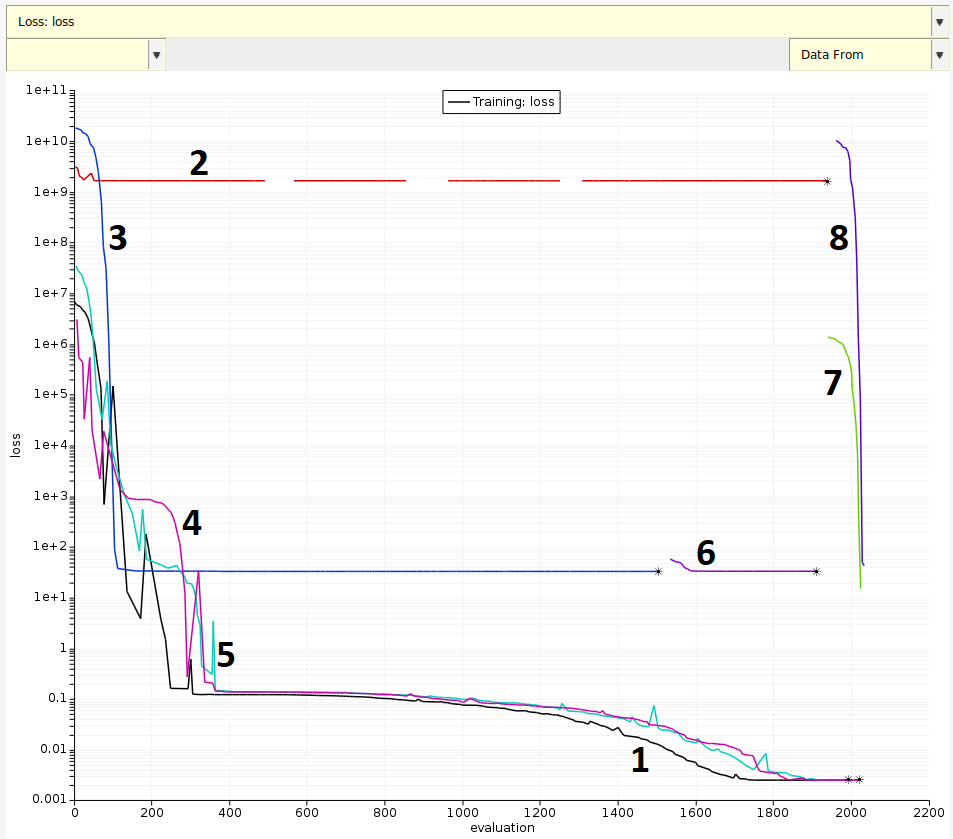
Fig. 5.3 Example development of multiple optimizers with random starts.¶
Your optimizers will behave a little differently, but hopefully you will see similar behavior.
Optimizer 2 started in a bad location and was barely able to improve on its starting value.
Optimizer 3 improved significantly on its starting value, but actually converged to the wrong minimum.
Optimizers 1, 4 and 5 all eventually found the correct minimum.
Optimizer 6, which started after optimizer 3 converged, started in quite a good value but was hardly able to improve on it, despite being far from the minimum.
Optimizers 7 and 8 were started very late and were not given time to develop before the exit condition of 5 converged optimizers was met and the optimization exited.
This simple example illustrates the importance of running multiple optimizations. There is no guarantee that a single optimizer (even if it looks like it has improved on its starting value) has actually found a good minimum. As the number of model parameters increases, this problem becomes even more pronounced.
5.4.1.1. Loss graphs with multiple optimizers¶
5.4.1.1.1. Global evaluation numbers¶
In Fig. 5.3, the loss value evaluated by each optimizer is plotted against a unique, ordered, global evaluation ID number. In other words, it is not the number of evaluations a single optimizer has used, but the total used by all optimizers up to that point.
This approach allows us to visualize how multiple optimizers are related in time. For example, we can see that optimizer 6 was started later in time than the first five.
The evaluation numbers are unique and appear consistently throughout the logs.
For example, consider the log for optimizer 2 (found at results/optimization/optimizer_002/training_set_results/running_loss.txt):
#evaluation training_set_loss log10(training_set_loss) time_seconds
000003  3200228859.254910 10.260 1.10
000009  3131651984.274525 10.258 2.33
000018  2942423641.003031 10.203 3.68
000024  2454079400.461060 10.129 4.45
This means that optimizer 2 has been logged 4 times, which corresponds to the 3rd, 9th, 18th and 24th overall calls. The loss function is logged whenever it becomes smaller, or by default every 10 local optimizer evaluations (this can be configured on the Details → Output panel).
Note
The default logging system prints global evaluation numbers. If you need local evaluation numbers, use the HDF5 logging architecture.
5.4.1.1.2. Failed optimization steps¶
Gaps can be seen in the trajectory for optimizer 2. These gaps represent invalid output from the optimizer. This can occur through crashed jobs, unstable parameter combinations, or non-physical results. Optimizer steps that violate constraints are also omitted from the trajectories.
5.4.1.1.3. Identifying optimizers¶
We have added optimizer numbers to the image above for ease of reference in the tutorial. To see the optimizer number yourself, mouse over the curve you are interested in. This will give you a pop-up of the form:
<(optimizer#)> loss: (eval#), (lossvalue)
If you would like to see just one optimizer you can click on the curve you would like to see, and the others will disappear. Click on it again to restore the original view.
To show a subset of optimizers:
2 4 7This will hide all the optimizer trajectories except the ones you have chosen.
To show all the trajectories again:
5.4.2. Using stoppers¶
In Fig. 5.3 we can identify two inefficiencies:
Optimizers 2 and 3 are clearly stuck in bad minima. They appear converged, but at loss values which are much worse than ones being simultaneously explored by optimizers 1, 4 and 5.
Optimizer 1, 4 and 5 end up converging to the same minimum. Multiple optimizers finding the exact same minimum is a waste of resources.
These problems can be solved with Optimizer Stoppers. Stoppers
are simple conditions which can be combined to form more complex stop criteria,
stop optimizers early if they are behaving poorly,
let you use computational resources more efficiently,
help you identify better minima within the same period of time
This managed parallel optimization approached was developed by Freitas Gustavo and Verstraelen (2021).
See also
For now we will set up Stoppers which directly address the 2 inefficiencies we identified above.
to open the input panel if it is not already open icon which will add a new Stopper
100.05The Current Function Value Unmoving Stopper will stop optimizers which are no longer significantly improving their function value and are exploring values which are worse than the best optimizer.
icon to add a second Stopper0.01The Max Interoptimizer Distance Stopper will stop optimizers which are close together (approaching the same minimum for example).
1 | 2This means that a stop will be triggered if the conditions of Stopper #1 or Stopper #2 are met.
Stopper
    Type CurrentFunctionValueUnmoving
    CurrentFunctionValueUnmoving
        NumberOfFunctionCalls 10
        Tolerance 0.05
    End
End
The CurrentFunctionValueUnmoving Stopper will stop optimizers which are no longer significantly improving their function value and are exploring values which are worse than the best optimizer.
Stopper
    Type MaxInteroptimizerDistance
    MaxInteroptimizerDistance
        MaxRelativeDistance 0.01
    End
End
The MaxInteroptimizerDistance Stopper will stop optimizers which are close together (approaching the same minimum for example).
StopperBooleanCombination 1 | 2
StopperBooleanCombination 1 | 2 means that a stop will be
triggered if the conditions of either Stopper #1 or Stopper #2 are
met. Stoppers are automatically numbered by the order in which they
appear in the input file.
You can combine Stoppers in logical and combinations too using the & symbol, and they can also be nested with parentheses.
For example, (1 | 2) & 3 means: Stop if Stopper #3 is true and either Stopper #1 or Stopper #2 is true.
Note
The or combination of all Stoppers is the default combination. We only entered it explicitly here to draw your attention to Stopper combinations. You could leave this unassigned in this example and achieve the same result.
Run the optimization.
multiopt2.paramsBelow is an example run we performed.
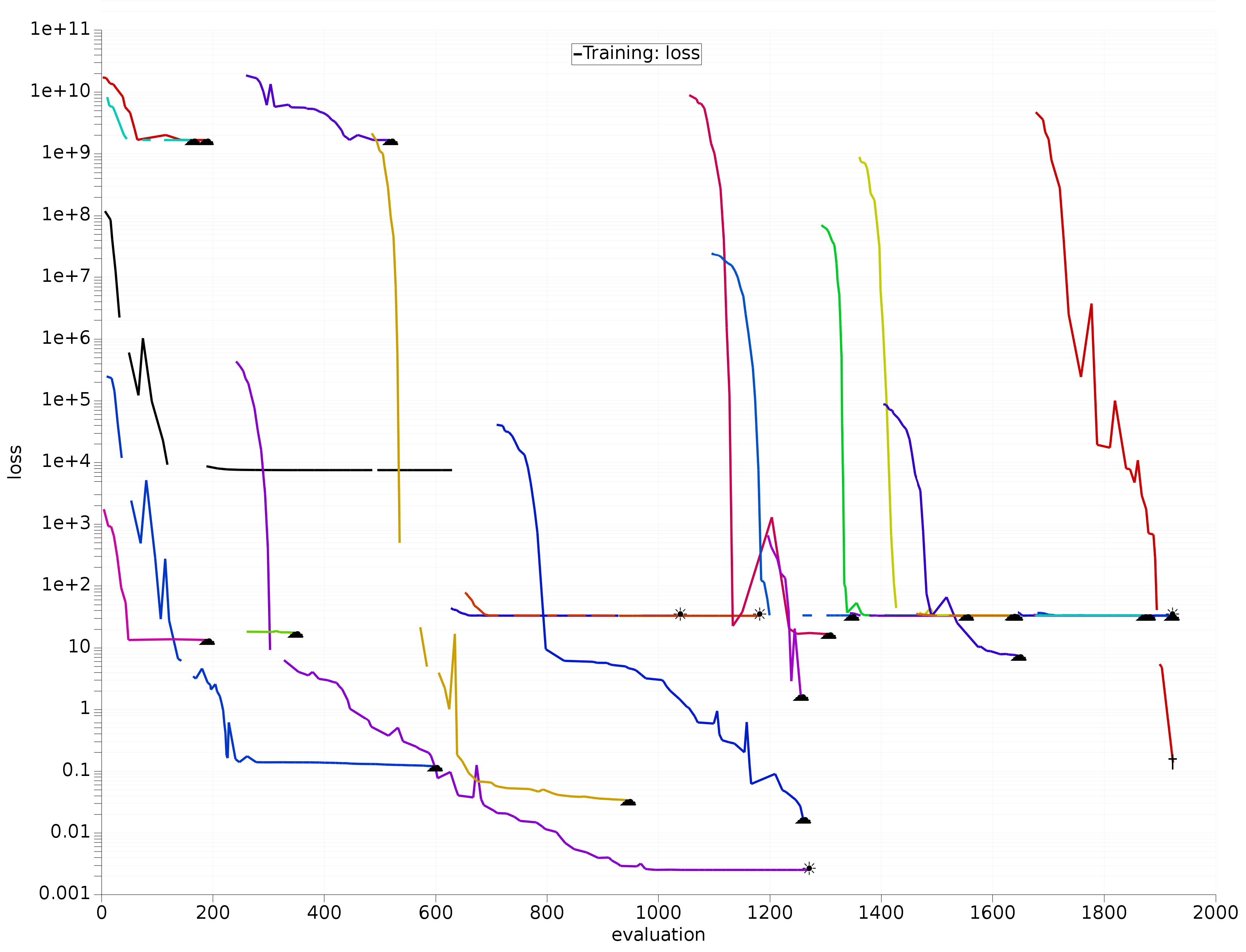
Fig. 5.4 Example development of multiple optimizers with random starts and stoppers.¶
In this figure you can see that the following optimizers were stopped:
flat optimizers which struggled to improve on their loss value (Current Function Value Unmoving)
optimizers approaching the same minimum as the best optimizer (Max Interoptimizer Distance)
Compare Fig. 5.4 and Fig. 5.3. The result of using Stoppers were:
starting many more optimizers within approximately the same number of function calls
global minimum was still found
the search was much more exploratory and our time was used more efficiently.
On a harder optimization problem like ReaxFF, this managed approach may allow you to find more (and hopefully better) minima than a simple parallel approach.
5.4.2.1. Loss graphs with stoppers¶
To show why optimizers have been stopped, icons are appended to the end of their trajectories:
Icon |
Description |
|---|---|
✳ |
Optimizer converged naturally |
▲ |
Optimizer stopped by Stopper |
† |
Job exit |
To get more details about the stop, you can mouse over the icon at the end of its trajectory.
5.4.3. Add a spawning limit¶
In Fig. 5.3 and Fig. 5.4 you can see optimizers which were started near the end of the optimization and given very little time to iterate at all.
You may want to limit the number of optimizers you start to
prevent optimizers from starting (spawning) near the end of the job, or
get a specific number of results.
This can be done with spawning controls.
to open the input panel if it is not already openControlOptimizerSpawning
MaxEvaluations 1500
End
The params_complete.in file included in the example files contains the input configuration for the optimization with Stoppers and spawn control.
Tip
This file can be loaded by the GUI if it is opened as the first file in ParAMS.
If you select one of the YAML files then params.in will be loaded instead.
This will stop new optimizers from starting after 1500 total function
evaluations, but it will not affect optimizers which are already working.
It is different from the Max Total Function Calls Exit
Condition as follows:
Spawning control |
Exit condition |
|
|---|---|---|
GUI Panel |
Options → Optimizer Spawning |
Main Optimization panel |
Input file block |
|
|
Triggered at #evaluations (this tutorial) |
1500 |
2500 |
Affects currently running optimizers |
No |
Yes (complete exit) |
Causes the job to exit |
Only if all optimizers stop |
Yes, always |
We previously specified to run at most 5 optimizers in parallel. By applying spawning control, fewer than 5 optimizers may run in parallel after iteration 1500.
multiopt3.params and run.Our example run is below where you can see that all optimizers were given enough time to develop, either by converging or reaching a stopper.
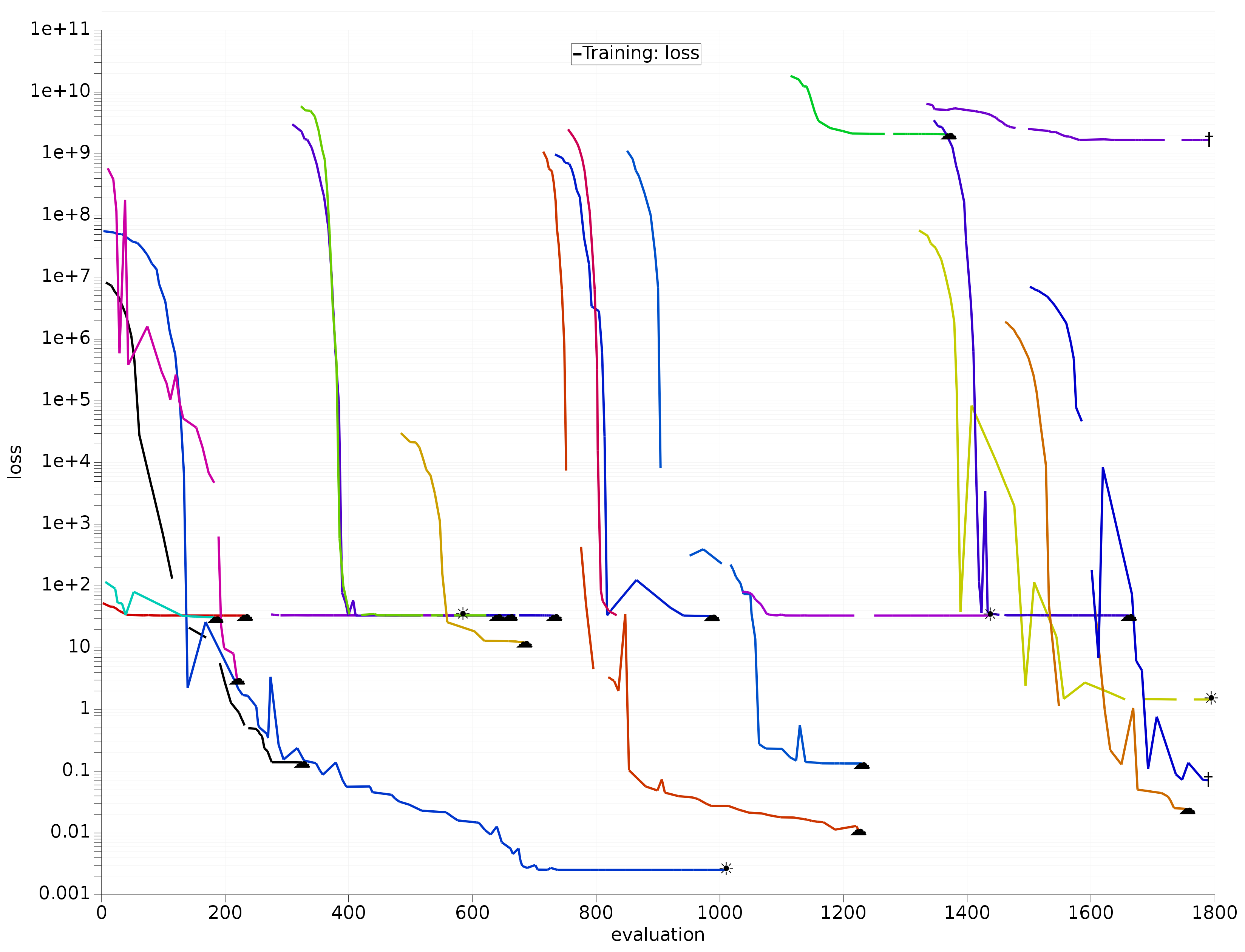
Fig. 5.5 Example development of multiple optimizers with random starts, stoppers, and spawn control.¶
5.4.4. Experiment with different optimizers¶
So far we only used the Nelder-Mead algorithm. However, you may want to
compare how different optimizers perform on a problem, and
see how different hyperparameter settings change performance.
For this we will remove the interoptimizer distance Stopper since we would like to see which optimizer is better at finding the minimum.
to open the input panel if it is not already open button for the Max Interoptimizer Distance Stopper
Next, we will add a second optimizer to the pool of available optimizers that can be used during the optimization:
to open the input panel if it is not already open button to add a new Optimizer0.158Optimizer
Type CMAES
CMAES
Popsize 8
Sigma0 0.15
End
End
The params_twotype.in file included in the example files contains the input configuration for this optimization using two different optimizers.
Tip
This file can be loaded by the GUI if it is opened as the first file in ParAMS.
If you select one of the YAML files then params.in will be loaded instead.
We now want to control when each optimizer type gets started. By default ParAMS will simply cycle through the set sequentially, which is usually a good choice.
For this tutorial, we will start several Nelder-Mead optimizers and then several CMA-ES optimizers in order to compare which performs better.
to open the input panel if it is not already open500OptimizerSelector
Type Chain
Chain
Thresholds 500
End
End
With this setup,
Nelder-Mead optimizers start before 500 global function evaluations
CMA-ES optimizers start after 500 global function evaluations
multiopt4.params and run.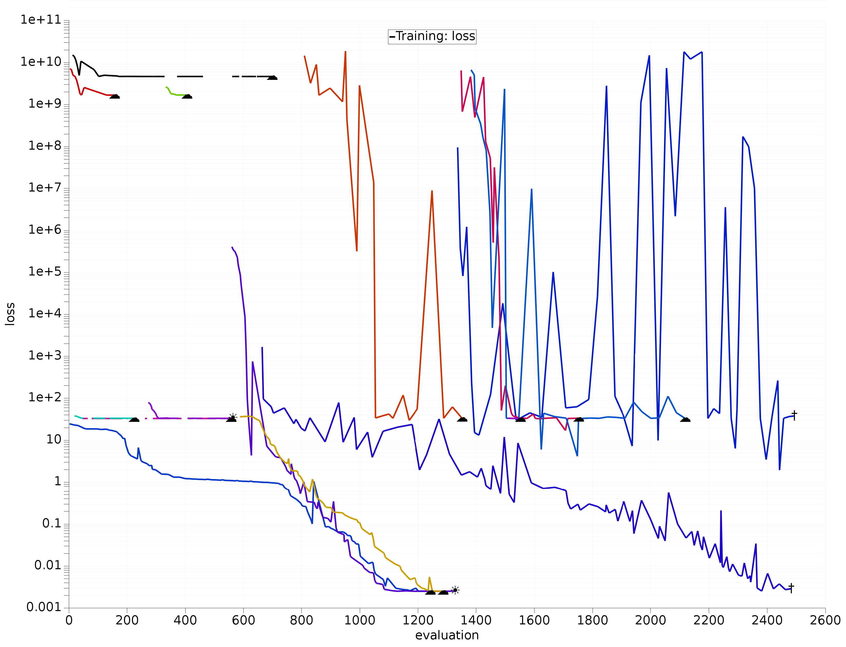
Fig. 5.6 Example development of multiple optimizers with random starts, stoppers, and different types of optimizers. All optimizers started before evaluation 500 are Nelder-Mead. All optimizers started thereafter are CMA-ES.¶
In our run we see that CMA-ES optimizers are much more exploratory than Nelder-Mead and oscillate quite wildly while Nelder-Mead attempts to go straight to a minimum. Of the 7 Nelder-Mead optimizers started here, only one found the global minimum. Of the 8 CMA-ES optimizers started, 3 found the global minimum. However, CMA’s exploratory nature can make it quite slow.
Tip
You can see what type an optimizer is in the results file by looking at: results/optimization/optimizer_xxx/opt_type.txt